Motion Primitives and Planning for Robots with Closed Chain Systems and Changing Topologies

(1)

University of Pennsylvania

ScholarlyCommons

Publicly Accessible Penn Dissertations

1-1-2013

Motion Primitives and Planning for Robots with

Closed Chain Systems and Changing Topologies

Steven Robert Gray

University of Pennsylvania, [email protected]

Follow this and additional works at:http://repository.upenn.edu/edissertations Part of theRobotics Commons

Recommended Citation

Gray, Steven Robert, "Motion Primitives and Planning for Robots with Closed Chain Systems and Changing Topologies" (2013).

Publicly Accessible Penn Dissertations. 757.

(2)

Motion Primitives and Planning for Robots with Closed Chain Systems

and Changing Topologies

Abstract

When operating in human environments, a robot should use predictable motions that allow humans to trust and anticipate its behavior. Heuristic search-based planning offers predictable motions and guarantees on completeness and sub-optimality of solutions. While search-based planning on motion primitive-based (lattice-based) graphs has been used extensively in navigation, application to high-dimensional state-spaces has, until recently, been thought impractical. This dissertation presents methods we have developed for applying these graphs to mobile manipulation, specifically for systems which contain closed chains. The formation of closed chains in tasks that involve contacts with the environment may reduce the number of available degrees-of-freedom but adds complexity in terms of constraints in the high-dimensional state-space. We exploit the dimensionality reduction inherent in closed kinematic chains to get efficient search-based planning.

Our planner handles changing topologies (switching between open and closed-chains) in a single plan, including what transitions to include and when to include them. Thus, we can leverage existing results for search-based planning for open chains, combining open and closed chain manipulation planning into one framework. Proofs regarding the framework are introduced for the application to graph-search and its theoretical guarantees of optimality. The dimensionality-reduction is done in a manner that enables finding optimal solutions to low-dimensional problems which map to correspondingly optimal full-dimensional solutions. We apply this framework to planning for opening and navigating through non-spring and spring-loaded doors using a Willow Garage PR2. The framework motivates our approaches to the Atlas humanoid robot from Boston Dynamics for both stationary manipulation and quasi-static walking, as a closed chain is formed when both feet are on the ground.

Degree Type Dissertation

Degree Name

Doctor of Philosophy (PhD)

Graduate Group

Mechanical Engineering & Applied Mechanics

First Advisor Vijay Kumar

Second Advisor Maxim Likhachev

Keywords

(3)

(4)

MOTION PRIMITIVES AND PLANNING FOR ROBOTS WITH

CLOSED CHAIN SYSTEMS AND CHANGING TOPOLOGIES

Steven R. Gray

A DISSERTATION

in

Mechanical Engineering and Applied Mechanics

Presented to the Faculties of the University of Pennsylvania in Partial

Fulfillment of the Requirements for the Degree of Doctor of Philosophy

2013

Vijay Kumar, PhD, Supervisor of Dissertation

Professor, Department of Mechanical Engineering and Applied Mechanics

Maxim Likhachev, PhD, Co-Supervisor of Dissertation

Research Assistant Professor, Robotics Institute

Jennifer Lukes, PhD, Graduate Group Chairperson

Associate Professor, Department of Mechanical Engineering and Applied Mechanics

Dissertation Committee:

(5)

Acknowledgements

While at the University of Pennsylvania, I worked on many different projects which

let me explore different aspects of robotics. To all those I worked with at Penn,

Carnegie Mellon, Willow Garage, Lockheed Martin, and other partner institutions

and organizations, thank you for helping me learn and experience so much.

I would like to thank my advisors, Vijay Kumar and Maxim Likhachev, for all of

their support and advice. Vijay is a dedicated advisor who has let me choose and

shape my involvement in the projects we worked on together. Max has always been

there to help me with questions and think through solutions to those issues that

inevitably crop up during implementation. I consider myself very fortunate to have

had Vijay and Max as mentors. Additionally, I would like to thank Mark Yim, George

Pappas, and Sachin Chitta for taking the time to serve on my dissertation committee.

I would also like to thank all my friends and colleagues in GRASP for making the lab

a great place to work and for making Philadelphia a great place to have spent these

past six years.

I am immensely grateful to my family for their love and support. My parents

(6)

accomplish whatever I set out to do. My wife, Danielle, has been there for me every

step of the way. She cheers me when I am down, lights a fire under my butt when I

(7)

ABSTRACT

MOTION PRIMITIVES AND PLANNING FOR ROBOTS WITH

CLOSED CHAIN SYSTEMS AND CHANGING TOPOLOGIES

Steven R. Gray

Vijay Kumar

Maxim Likhachev

When operating in human environments, a robot should use predictable motions

that allow humans to trust and anticipate its behavior. Heuristic search-based planning

offers predictable motions and guarantees on completeness and sub-optimality of

solutions. While search-based planning on motion primitive-based (lattice-based)

graphs has been used extensively in navigation, application to high-dimensional

state-spaces has, until recently, been thought impractical. This dissertation presents methods

we have developed for applying these graphs to mobile manipulation, specifically for

systems which contain closed chains. The formation of closed chains in tasks that

involve contacts with the environment may reduce the number of available

degrees-of-freedom but adds complexity in terms of constraints in the high-dimensional state-space.

We exploit the dimensionality reduction inherent in closed kinematic chains to get

efficient search-based planning.

Our planner handles changing topologies (switching between open and

closed-chains) in a single plan, including what transitions to include and when to include

(8)

chains, combining open and closed chain manipulation planning into one framework.

Proofs regarding the framework are introduced for the application to graph-search

and its theoretical guarantees of optimality. The dimensionality-reduction is done

in a manner that enables finding optimal solutions to low-dimensional problems

which map to correspondingly optimal full-dimensional solutions. We apply this

framework to planning for opening and navigating through non-spring and

spring-loaded doors using a Willow Garage PR2. The framework motivates our approaches

to the Atlas humanoid robot from Boston Dynamics for both stationary manipulation

(9)

Chapter 1 Introduction

Interacting with objects in the environment is becoming increasingly important in

robotics. Robots are making inroads into human environments, from cleaning to

patient care [37, 45, 93]. They are moving beyond the rigidity of assembly lines and

fixed, repetitious motions [53, 94]. However, to effectively interact with the world

around them, including human environments, robots must be able to plan for situations

in which multiple contacts are made with the world. Additionally, when operating in

human environments, a robot should use predictable motions that allow humans to

trust and anticipate its behavior. Heuristic search-based planning offers predictable

motions and guarantees on completeness and sub-optimality of planned trajectories.

While search-based planning on motion primitive-based (lattice-based) graphs has been

used extensively in navigation, application to high-dimensional state-spaces has, until

(14)

graphs to mobile manipulation, specifically for systems which contain closed chains.

The formation of closed chains in tasks that involve contacts with the environment

may reduce the number of available degrees-of-freedom but adds complexity in terms

of constraints in the high-dimensional state-space. We exploit the dimensionality

reduction inherent in closed kinematic chains to get efficient search-based planning.

1.1 Background

As the complexity of our robotic platforms increases, so does the need to plan

in high-dimensional state-spaces. As little as a decade ago, low degree-of-freedom

wheeled ground vehicles were dominant; now humanoid robots and mobile manipulation

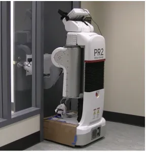
platforms abound. Two popular platforms, the Willow Garage PR2, with its holonomic

wheeled base and dual arms (for a total of 20-degrees-of-freedom), and the humanoid

HUBO, with 38-degrees-of-freedom, are shown in Figure 1.1.

Probabilistic sampling-based planning methods have come to the fore as a tractable

means of searching high-dimensional spaces. However, they have a cost: these methods

trade guarantees on solution completeness (with respect to geometric algorithms) and

optimality (with respect to search-based algorithms) for speed, and must settle for

probabilistic completeness guarantees. While RRT∗ and related works seek to recover

path optimality, they may only do so in an asymptotic fashion; as the number of

samples approaches infinity, they approach the optimal solution [56, 83]. Lately, there

(15)

(a) (b)

Figure 1.1: The Willow Garage PR2 (a) with 20-degrees-of-freedom and the Korea

Advanced Institute of Science and Technology (KAIST) HUBO (b) with

38-degrees-of-freedom are widely-used robotics platforms which require planners capable of handling many

(16)

Search-based planning is being applied to higher degree-of-freedom systems than ever

before, as will be discussed in Chapter 2.

Planning for navigation, whether for field robots or robotic manipulators, typically

involves planning through free space without additional constraints. Even in mobile

manipulation literature, the common paradigm is to plan to get an end-effector near

an object to manipulate, form the appropriate pre-grasp pose, approach the object

to grasp, then move with the object attached, again planning without constraints

[20, 22, 99, 111]. Other works have introduced constraints on manipulated object

poses [7, 9]. However, there are instances when planning for mobile manipulation

cannot be reduced to a series of open-chain planning problems. For instance, when

interacting with an object constrained by or attached to the world in some way.

Examples include opening doors and drawers, using levers and valves, and pushing

objects along a track.

1.2 Motivation and Contributions

This thesis will demonstrate that search-based algorithms are applicable to systems

with many degrees-of-freedom involving closed chains. The closed chains often arise in

the form of contacts with the world, such as in mobile manipulation. Towards that end,

we present a planning framework for search-based planning for mobile manipulators

with changing system topologies; the systems contain closed chains, open chains, and

(17)

doors and is used to motivate our approach to bipedal locomotion. Door opening is

an example of planning to manipulate an object along a constrained trajectory. Both

tasks involve making and breaking closed chains.

First, Chapter 2 will provide an overview of the current state of the art in

motion planning, planning for closed chains, and planning for mobile manipulation.

Hierarchical planners and motion primitive-based planners will be covered. The

algorithms involved span the gamut from deterministic, geometry-based planners to

random sampling-based planners with probabilistic completeness guarantees to

graph-based planners with their bounds on suboptimality of solutions. Additional literature

pertaining to applications in later chapters will be discussed in those chapters.

In this thesis, we use search-based-planning algorithms. Chapter 3 begins with an

overview of search-based planning, from Dijkstra’s algorithm up to modern motion

primitive-based approaches. This includes an overview of the A∗, Weighted A∗, and

Anytime Repairing A∗ algorithms. We discuss lattice-based graphs, connected by

motion primitives. Further, Chapter 3 provides descriptions of closed chains, systems

in which they are likely to appear, and what constraints they impose.

Chapter 4 introduces our planning framework for handling open chains, closed

chains, and transitions between them, all in a single planning instance, maintaining the

completeness and optimality guarantees which would have been lost or weakened in a

hierarchical planner. Theoretical guarantees are mentioned along with the necessary

(18)

provided.

Chapter 5 covers application of our framework to the task of opening spring-loaded

and non-spring-loaded doors using a mobile manipulator with a holonomic base. The

door is constrained by its attachment to the world via revolute joint and may only

move along a 1-D manifold, though it may move in either direction along that manifold.

The robot must move its base to open the door and pass through the doorway. It may

also switch between contacts with the door during planning and is allowed to contact

the door with either arm, the base, or nothing at all.

Finally, Chapter 6 describes our approach to walking for a humanoid. We detail

our control framework for the DARPA Robotics Challenge, specifically a balancing

controller which has been extended to support quasi-static walking. In the double

stance phase, the lower body forms a closed chain, while the single stance phase is an

open chain. Planning for the humanoid involves abstractions for the complexity of

kinematic chains from the pelvis to each foot. On that note, our planning framework

inspires our work on walking, but the system is complex and the required assumptions

and thus the guarantees of the framework do not apply directly. Our planning and

control are able to successfully negotiate difficult terrain with hills and scattered

(19)

Chapter 2 Literature Review

2.1 Background on Motion Planning

Motion planning difficulty depends on the dimensionality of the system and the

constraints on the motion. Exact algorithms, which guarantee a solution when one

exists and return failure when one does not, are limited to low-dimensional

config-uration spaces due to computational complexity. For instance, the most efficient

exact algorithm has exponentially increasing complexity in dimensionality [17]. When

considering the history of motion planning, we see that with exact methods

infea-sible, it was necessary to sacrifice exact completeness in order make the planning

problem tractable. Discretization of dimension and configuration parameters was

introduced. In general, algorithms based on an approximated cell decomposition of

(20)

discretization size. In fact, narrow passageways smaller than the discretization size

are guaranteed to be missed. Efficient heuristic algorithms have been developed based

on the potential field approach [58]; these perform gradient descent on the potential

field and may become trapped at local minima. Thus, the design of the potential

function is crucial, but difficult for non-convex and high-dimensional spaces. All of the

above approaches are applicable in practice to systems involving only a few variables,

typically four or less.

Sampling-based planners, satisfying a weaker form of completeness but capable of

handling high-dimensional configuration spaces, were introduced in the 1990s [57, 64].

These planners, probabilistic roadmaps (PRMs) and rapidly-exploring random trees

(RRTs) guarantee probabilistic completeness; the planners sample randomly (or

in a biased random fashion) from the configuration space. Such planners are not

guaranteed to find a solution if it exists, often the case in the narrow passage problem,

though variants have been introduced to handle such cases. There is also a drive to

derandomize the sampling to improve coverage properties [63].

Lattice-based planners, used in this thesis, allow for planning as graph search.

Such planners allow us to leverage results in graph search literature (A∗, D∗ and their

variants), previously applied to cell-decomposition methods. These methods have

recently been shown to be applicable to high-dimensional state-spaces, as discussed in

(21)

2.2 Planning for Generic Closed-Chain Systems

A number of planning methods exist specifically for closed kinematic chains. The

works discussed below address planning for closed chain systems consisting of rigid

links in 2-D (revolute and prismatic joints only) or 3-D (also includes ball joints).

Complete planners suffer from high computational complexity and difficult

im-plementations. Some works, such as [103], are complete, but the path returned is

not optimal by any metric. The cited work is valid for closed kinematic chains with

spherical joints and will use at most n−2 accordion moves to reach the desired configuration. The accordion moves are not optimal with respect to distance traveled

nor any other metric. These works do not handle self-collisions or obstacles. An

extension allowing point obstacles is limited to planar chains [67].

Early sampling-based methods for closed-chains were slow because the vast majority

of generated samples did not satisfy the loop-closure constraints and so were rejected.

A later sampling method, [112], applied to closed chains of a single cycle. It broke the

closed chains into sub-chains, one of which used standard random sampling techniques,

and the other which was populated using inverse kinematics to enforce the closure

constraints. This method was applied to mobile manipulators and employed a

two-stage PRM strategy. The first two-stage was generating a PRM for the manipulator at a

single base location, and the second stage was replicating the PRM at different base

locations and connecting them.

(22)

broken apart and gradient descent applied to minimize the sum of squares Euclidean

distances between joints that should be collocated to satisfy the kinematic closure

constraint. While samples could thusly be modified to satisfy the closure constraint,

this was a time-consuming endeavor. In [101], the authors propose planning with

reachable distances, precomputing and sampling directly from the subspace that

satisfies the closure constraints. Closed chain systems are represented as a hierarchy

of sub-chains; the corresponding reachable range of each can be computed using the

triangle inequality. The method can be applied to most sampling-based planners, such

as PRMs and RRTs. It has so far been applied to abstract chains in simulation.

The sampling-based works above have been applied to mobile manipulators, but

do not allow for constraints on the motion of a manipulated object. The geometric

methods have not been applied to mobile manipulation and cannot, for example,

account for nonholonomic constraints of a robot base.

2.3 Application to Mobile Manipulators

As a central idea of this thesis is planning for closed-chain systems with specific

application to mobile manipulation, we include an overview of other methods used in

that field.

The idea of decomposing the motion of mobile manipulators into mobility and

manipulation dates back to the first discussions of such systems in the 1980s. In [18],

(23)

and end-effector configurations were considered separately, and the optimization

problem was solved for a sequence of manipulator and base configurations which

minimized the cost function. Controls-based approaches have been used to drive a

robot base in a manner that enables following specified end-effector trajectories [35].

Given a path for the end-effector, a feasible path is planned for the base such that

the end-effector trajectory is always in the dexterous workspace. In this work, the

dexterous workspace is always projected onto the ground plane, ignoring the height.

Stability for the base and end-effector trajectory-following controllers is proven.

Finding the appropriate base position for manipulation tasks is not a trivial

problem. Some work has applied probabilistic methods like rapidly-exploring random

trees and probabilistic roadmaps to plan motions for mobile manipulators taking

inverse kinematics and base position into account. For instance, [77] addresses the

problem of motion planning along a specified end-effector path for a mobile manipulator

with a nonholonomic wheeled base and kinematically redundant manipulator. For a

given initial configuration, a path is assigned and a feasible solution generated using

probabilistic methods. Redundant variables are chosen in advance; when sampling,

values for these redundant variables are randomly generated, then the remaining

variables are solved analytically. The redundant variables may also be generated by

forward-integrating the equation of motion for the system using a random

pseudo-velocity. Unlike our work, there are no optimality guarantees and only probabilistic

(24)

Probabilistic roadmaps (PRMs) have been used to solve multiple-query problems

for mobile manipulators. Similar to RRTs, randomly sampled states are checked for

feasibility, then connections between states are evaluated for feasibility. Unlike RRTs,

a tree structure is not required; cycles are allowed and in fact add robustness. Work

has gone to speeding this process up by only evaluating necessary connections between

states (those required as the graph search is in progress), called Lazy PRM [11]. Lastly,

it has been recognized that the probabilistic sampling is often unnecessary, leading to

regularly-sampled versions, called LRMs [63].

In [104], solutions for dual-arm manipulation tasks are addressed for a fixed-base

robot. First, the robot’s reachability workspace is precomputed; it is represented

by voxels in 6-D pose space and each voxel contains a probability of successfully

answering an inverse kinematics (IK) query, i.e, solving for joint angles that produce

the desired end-effector pose. Gradient descent is used to find a local maximum

in the reachability space and combined with random sampling of free parameters.

Then RRT-based motion planning algorithms are applied, interleaving finding IK

solutions with searching for a collision-free trajectory. The work of [114] analyzes the

manipulator reachability by discretizing the workspace with a regularly spaced spheres.

On each sphere n-points are uniformly distributed, then frames are generated for each point on the sphere and serve as the tool center point for the inverse kinematics of

the robot. Cross-correlation is used to decide the best base location for carrying out a

(25)

the spheres. In this work, the trajectory is required to be completely contained in the

reachable workspace from a specific base location.

Berensonet. al introduce constrained bi-directional RRT for planning in

configura-tion spaces with multiple constraints [10]. Pose constraints are handled by projecting

sampled states onto configuration-space manifolds. The most common projection

tech-nique is the the Jacobian pseudo-inverse, in which the required workspace displacement

to place the configuration back onto the manifold boundary is first calculated, then

mapped into the joint space of the manipulator using the Jacobian inverse for square

Jacobians or the Moore-Penrose pseudo-inverse for non-square Jacobians. The planner

is able to handle moving heavy objects using sliding surfaces which support part of an

object’s weight. Dragging an object along a surface becomes an additional constraint

manifold; if the object is not near a sliding surface but is too heavy to be lifted by

the manipulator, the configuration is rejected. The advantage of our search-based

method over this is that we may use the constraints to reduce the dimensionality of

the state-space we are searching; the constraints enable a faster search.

CHOMP [92] is a trajectory optimization method that creates a naive initial

trajectory from start to goal (unconstrained, it does not need to be a feasible trajectory),

then runs a modified gradient descent on the cost function. The cost function typically

has two components, one which is a cost for points along the arm which increases

as they approach obstacles (this requires precomputation of a signed distance field)

(26)

to check the output of CHOMP for feasibility, i.e., being collision-free. The result of

CHOMP is dependent on the initial trajectory given, as it may get caught in local

minima. STOMP [54] is a similar approach which adds random noise to attempt to

avoid local minima.

In contrast, [98] presents a trajectory optimization method which combines

sequen-tial convex optimization with a novel formulation of the collision avoidance constraint

considering swept volumes. Rather than requiring precomputation of a signed distance

field for the environment, this work requires either an approximate convex

decomposi-tion or a simplified mesh. Results compare favorably to CHOMP and STOMP. The

work of Vernazaet al. focuses on identifying the low-dimensional Lagrangian structure

of physical systems and applying this knowledge to aid in high-dimensional motion

planning [105–107]. The algorithm learns and exploits the structure of holonomic

motion planning problems using spectral analysis and iterative dynamic programming

and is able to solve problems in higher dimensions than known methods for optimal

motion planning. The quality of solutions found compares favorably to those obtained

via sampling-based planning and smoothing.

RRT∗ is a recent development building upon RRT which converges to an optimal

path as the number of samples tends to infinity. It adds a cost function which is used

to calculate cost between vertices. When adding vertices to the tree, the edges are

rearranged such that each vertex is reached using a minimum cost path from the

(27)

degrees-of-freedom by combining RRT∗ with the Ball Tree Algorithm. Other attempts

to use probabilistic planners on costmaps include [6]. In this work, transitions to

an increased cost state were allowed with a probability that depended on a thermal

energy analog. When many subsequent expansions were rejected, the energy increased.

This work does not provide guarantees on path optimality, but has a tendency to

explore connected low-cost regions first and as such is appropriate for what the authors

deem cost space chasms, narrow regions of low cost surrounded by higher cost, often

of lower-dimensionality than the state-space and so unlikely to be found by naive

sampling.

Hierarchical planning schemes have been proposed to reduce complexity by

sepa-rating planning into smaller, simpler problems. Typically, a high-dimensional local

planner is combined with a low-dimensional global planner. The typical benefit of a

multi-level scheme is a significant reduction in planning time. Local planners have

been implemented using various techniques, including reactive obstacle avoidance [102]

and dynamic windows [15, 85]. While these types of planners can result in difficulties

with suboptimality and mismatches between the local and global levels, our approach

avoids these problems altogether by generating optimal plans in a low-dimensional

space that maps to much higher-dimensional optimal solutions. Our representation

has an additional advantage of incorporating a parameter to describe the contact

state of the mobile manipulator and object being manipulated, allowing one plan to

(28)

optimality.

2.4 Motion-Primitive Based Graph Planning

A key motivation of this thesis is to utilize lattice-based search for mobile manipulation.

The advantage of search-based plans is bounded solution suboptimality, as well as

determinism of solutions and completeness with respect to the discretization.

Searching motion primitive-based graphs has been applied to a variety of planning

problems in robotics, including navigation problems [65]. Specifically, this work

included planning dynamically-feasible maneuvers for vehicles at high speeds over

large distances. Motion primitives searches have also been used for planning trajectories

for UAVs [61, 68].

Formulation of motion primitives is key in [88]. In order to allow backward searches

such as D∗, it is necessary to make sure the motion primitives can be connected forwards

and backwards. Towards this end, they are constrained to begin and end on regularly

discretized grid-cell centers. Motion primitives are pruned to generate near-minimal

spanning action spaces by representing longer primitives as combinations of other

primitives when possible. The work has also been extended to handle dynamics [89]

by solving the corresponding two-point boundary value problem. The method has

been shown to be valid for low-dimensional systems like wheeled vehicles, and has

recently been extended to quadrotors [90].

(29)

high-dimensional problems, specifically manipulation problems [23]. Planning times are

lessened by combining informative but quickly computable heuristics (a Dijkstra

search over the voxelized 3-D workspace), a small number of motion primitives, and an

anytime, incremental graph search, Anytime Repairing A∗ (ARA∗). An extension [25]

incorporates motion primitives with variable dimensionality; these lower-dimensional

primitives move a subset of the joints and are only used when near the goal end-effector

position. Motion primitives which use inverse-kinematics to directly move from the

current position to the goal are also used when near the goal. Additional constraints

present in two-arm manipulation have been used to plan in a lower-dimensional

graph [24]. A similar approach is used by [21], but their system lacks the ability to

push and pull spring-loaded doors or make and break contact points with the doors.

More recently, experience graphs have used results from previous searches have been

incorporated to bootstrap solutions for new queries [86, 87].

Recent work has also been conducted on search-based planning with adaptive

dimensionality [38, 39]. This uses the intuition that while planning in full-dimensional

state-space is sometimes necessary, for large portions of the robot’s workspace it is not.

An adaptive-dimensional state-space and corresponding transition set is iteratively

constructed that that consists mainly of low-dimensional states and transitions, using

high-dimensional states only where necessary to ensure a feasible path. We incorporate

this approach in our work on mobile manipulation with closed chains.

(30)

algorithm [110]. Instead of planning for all robots in a configuration space containing

the union of all robot configuration spaces, each robot is planned for separately. The

configuration spaces are appended only if the robots are found to interact. In a process

termed subdimensional expansion, the algorithm searches a lower-dimensional graph

embedded in the full graph representing all the robots. Only when robots are found

to interact are higher-dimensional state transitions back-propagated.

In this thesis, we consider a variety of closed-chain mobile manipulation tasks,

including opening doors. This thesis represents the first work, to the author’s

knowl-edge, to incorporate transitions in system topology into search-based planning with

motion primitives. The additional constraints from closed-chains are used to reduce

system dimensionality in regions where the topology includes closed-chains, enabling

efficient search. In contrast with the works above, the planning framework herein

handles the transitions between open and closed chains in a single plan, including

what transitions to include and when to include them. It does so while maintaining

completeness and optimality guarantees over the entire plan, and the results share the

(31)

Chapter 3 Preliminaries

3.1 Graph Search

In this thesis, motion planning problems are represented by graph searches. Given a

finite graph, we need an efficient way to search it for a solution path. We will now

provide a brief review of graph search methods. We note that our planning framework

with its dimensionality reduction is independent of the graph search chosen, though

the specific guarantees of solution optimality do depend on the properties of the chosen

search method.

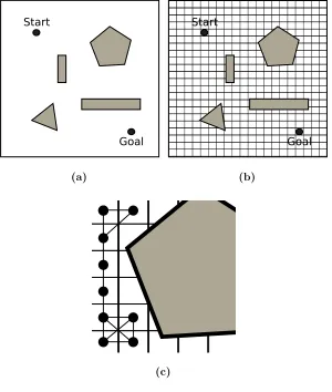
Depending on the search space, the easiest method for constructing a graph is to

discretize the state-space. For example, considering the 2-D search space in Figure 3.1,

we can easily uniformly discretize the space, yielding a grid. Each discretized state

(32)

Start

Goal

(a)

Start

Goal

(b)

(c)

Figure 3.1: A 2-D state-space example. A configuration-space map (a) is uniformly

(33)

to another. Each edge has a weight which corresponds to the distance between cells.

It is easy to envision using a 4- or 8-connected grid representation for the discretized

space, as shown in the close-up in Figure 3.1(c).

Regardless of underlying representation, we discuss the planning problem as a

graph, G= [S, T], where S is the vertex set and T is the edge set. We define a set of transitions T ={ai,j|si, sj ∈S}, whereai,j is a transition from state si to state sj.

Each transition is associated with a non-negative costc(ai,j), also written as c(si, sj).

The objective of the planner is to find the least-cost path in G from start state sstart

to goal state sgoal. Let π(si, sj) denote a path fromsi to sj, and let π∗(si, sj) denote

the least cost path. The path cost is the sum of the transitions along the path,

P

i,j∈πc(ai,j), denoted asc(π(si, sj)).

3.1.1 Dijkstra Search

Dijkstra’s algorithm [33] solves the single-source shortest path problem for a graph

with non-negative edge weights. The g-value of a given state, g(s), represents the current lowest cost path to reach that state. The search is initialized withg(sstart) = 0,

(34)

theOP EN set. The process repeats until g(sgoal) is updated. The least cost path can

be reconstructed by working backwards from the goal, always choosing the predicate

state with the lowest g-value plus transition cost. Visualized on a 4 or 8-connected grid, Dijkstra’s algorithm can be likened to a wavefront propagating outward from

the start location.

Dijkstra’s Algorithm

g(sstart) = 0, all other states set to g(s) =∞

OPEN = {sstart}

while g(sgoal) ==∞ do

remove s with smallest g(s) from OPEN

for each successor s0 of s do if g(s0)> g(s) +c(s, s0) then

g(s0) =g(s) +c(s, s0)

Insert s0 in OPEN if not already present

3.1.2 A

∗

Algorithm

A∗ search is a popular graph search algorithm [46], improving upon Dijkstra’s algorithm

by utilizing a heuristic to focus the search toward the goal. The search introduces the

h- and f-values for a given state, where the h-value is the heuristic estimate of the cost to reach the goal and f(s) =g(s) +h(s). The search is very similar to Dijkstra, except (1) the state removed from the OP EN set each iteration is now the one with the lowestf-value and (2) thef-value is updated when theg-value is updated. The

h-values must be an underestimate of the least cost path from the current state to the goal (admissibility) in order to ensure that the algorithm returns the optimal path.

(35)

That is, for any two states where s0 is a successor of s, h(s)≤c(s, s0) +h(s0).

A∗ Algorithm

g(sstart) = 0, all other states set to g(s) =∞

OPEN = {sstart}

while g(sgoal) ==∞ do

remove s with smallest f(s) from OPEN

for each successor s0 of s do if g(s0)> g(s) +c(s, s0) then

g(s0) =g(s) +c(s, s0)

f(s0) = g(s0) +h(s0)

Insert s0 in OPEN if not already present

3.1.3 Weighted and Anytime Variants

The weighted version of A∗ works by biasing the sampling of new states toward the

goal. For a given admissible heuristic function, multiplying the heuristic by a constant

>1 and then performing the search as usual produces a solution with cost at most

times the least cost solution [82]. In many domains, using the inflated heuristic greatly reduces the number of states expanded by the search before finding a solution.

While A∗ is able to find optimal plans, it can fail to find solutions when deliberation

time is limited. Anytime planners, on the other hand, aim to find the best plan they

can in the time allowed [28]. A (possibly) highly suboptimal plan is found and then

improved and until either times runs out or the optimal solution is recovered.

In this thesis work, we have chosen to use an anytime heuristic search algorithm

called Anytime Repairing A∗ (ARA∗) [66]. The algorithm has control over the

(36)

property: it uses a loose bound to quickly find an initial solution, then tightens the

bound progressively as time allows. Given enough time, it arrives at the optimal

solution. ARA∗ reuses previous search efforts as it reducesand, thus, is more efficient than other anytime search methods. In comparison, a similar method called Anytime

A∗ does not control directly (aside from setting the maximum during the first search) [115]. Instead, it continues to expand and re-expand states after the first

solution is found by pruning states with f-values larger than the best cost solution so far.

3.2 Lattice State-Space

A state lattice, as described in [88], is a discretization of the configuration-space into a

set of states and the connections between those states. Unlike the simple 8-connected

grid representation of Figure 3.1, connections in the state lattice are required to be

feasible motions of the system. Thus, any solution found while searching a lattice

graph will also be feasible; the planner does not need to consider differential constraints

directly.

The searches of this thesis are applied to regular lattices of states. Regularly

sampled lattices provide translational invariance, in that a control or motion primitive

connecting two states arranged in a certain way will also connect all other pairs of

states arranged in the same way. Starting at a given location and applying the set of

(37)

a roadmap or graph containing all trajectories possible given the discretization and

choice of controls. The controls do not need to connect all adjacent states in the

discretized space, but it is required that the states they connect are separated by

multiples of the discretization value. These controls can be precomputed offline and

stored as a canonical set of allowed motions. Barring obstacles, these motions encode

the connectivity of the search space.

Motion primitives are defined as the smallest feasible motions that connect the

discretized states in the graph. When planning a kinematic path, they are defined

as small, kinematic displacements able to be tracked by the controller. Such is the

case in [23–25]. When planning a kinodynamic path, the primitives correspond to

known control inputs. Motion primitives can be designed by sampling the control

space. Most such works attempt to do so in such a way as to result in good sampling

in state-space in terms of discrepancy, dispersion or path diversity [13, 36, 44, 81].

In general, designing primitives this way is difficult due to the complexity of the

relationship between the robot’s control-space and state-space given the constraints

upon the system. Finding control inputs that drive the system from one state to

another can also be approached as solving a two-point boundary value problem for

systems where that is possible [88, 89].

Similarly to how the state-space is discretized, we can think of discretizing the

continuum of motions available to the system at a given state. This discrete set of

(38)

a wider variety of motion primitives and increased planning times. Smaller primitives

may help the planner find paths in narrow passageways, while longer primitives

may have faster planning times because fewer expansions are required. Ideally, the

action space for each state in the lattice would contain a sufficient variety of motion

primitives that every possible feasible path through the lattice could be constructed

by combining sequences of these actions. Realistically, including a large number

of primitives increases the branching factor of the graph to be searched and thus

negatively affects the time required for each expansion, which is proportional to the

total number of primitives. The best choice is often domain-dependent.

3.3 Closed Chains

A closed chain refers to a linkage whose kinematic structure contains one or more

cycles. Compared to an open chain of the same number of links, closed chains have

fewer degrees-of-freedom due to loop closure constraints. Namely, the product of all

frame transformations around the chain must yield the identity tranformation.

T1· · ·Tn =I

An open chain is considered kinematically redundant if it has more than the

minimally required degrees-of-freedom to span the space. For planar manipulators,

this value is 2; for spatial manipulators, it is 6. Consider a closed chain with one link

(39)

be able move; the valid motions of the closed chain comprise the self-motion manifold.

Internal motions are those motions along the self-motion manifold and must satisfy

J(θ) ˙θ =0

where J is the Jacobian and θ the vector of joint angles.

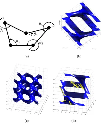
Consider, for example, a linkage consisting of 5-revolute joints with parallel axes

of revolution as shown in Figure 3.2(a). This planar 5-R linkage is kinematically

redundant and has 2 degrees-of-freedom taking the loop closure constraint into account.

If the linkage is equilateral, the configuration-space will look like Figure 3.2(b). For

visualization, the configuration-space has been plotted as a function of three of the

linkage joint angles, though it is actually a 2-D manifold. This manifold is the

self-motion manifold; any trajectory along it will satisfy the loop closure constraint.

Ignoring joint limits and self-collisions, the configuration-space can be endlessly

replicated, forming a complicated structure without discontinuity but with numerous

holes and thus many possible paths in different homotopy classes.

Because the space of valid configurations is a 2-D manifold, there is effectively no

chance of randomly sampling a valid configuration if sampling for all 5 joint angles.

There are methods that address this by breaking the closed chain into sub-chains and

only sampling for one of them. Because there are 2 degrees-of-freedom in this chain,

the active sub-chain will have 2 degrees-of-freedom and can use standard random

sampling techniques, while the passive sub-chain with 3 joints and will be solved using

(40)

(a) (b)

(c) (d)

Figure 3.2: Example showing the configuration-space of a planar, equilateral 5-R linkage

(a). The configuration-space is plotted as a function of the first three linkage joint angles.

The robot has two degrees-of-freedom and so the configuration-space is a 2-D manifold, with

black lines indicating stationary configurations (b). Ignoring joint limits and collisions, the

configuration-space can be replicated endlessly (c). Standard planning methods, such as

(41)

to sample directly in the space that satisfies the closure constraints [101] or to drive

the full-dimensional samples to the constraint manifold [6, 113].

In screw theory, a stationary configuration occurs when any k joint screws belong to a screw system of order less than k where k must be less than the number of joints in the chain and greater than 1 [60]. In case of the 5-R example, stationary

configurations occur when 3 or 4 of the joints are coplanar (though only 3 can be

coplanar if the linkage is equilateral). Stationary configurations are shown with black

lines in Figure 3.2(b). When 3 joints are coplanar, they have an instantaneous mobility

of 1, and the other two joints are constrained so they only have one independent

degree-of-freedom. Thus, if only those 2 joints were actuated, it would be impossible

to navigate the control singularity. When 4 joints are coplanar, the remaining joint is

transitorially inactive and cannot be used to control the robot through the singularity.

Thus, when actuating closed chains, choosing which joints to actively control and

which to make passive is very important.

Closed chains often arise in the form of contacts with the world, such as in mobile

manipulation. When such systems makes and break contacts, they transition between

open and closed chains. Bipedal walking is one example, in which the ground becomes

the link which closes the chain formed by the pelvis and legs. When a bipedal robot

is pushing against a wall with both hands, multiple closed chains arise; from each

hand to each foot, hand to hand, and foot to foot. All these chains are closed by the

(42)

Chapter 4 Planning Framework for Closed

Chains and Systems with

Changing Topologies

Motion primitive-based graph planning in high-dimensional systems is time consuming

as planning times increase exponentially with increasing dimensionality. This is

particularly a problem for mobile manipulation where the number of

degrees-of-freedom is quite large. In addition, contacts between the robot and the environment

result in the formation ofclosed chain linkages. A closed chain linkage is one whose

kinematic structure forms a cycle. Such cycles introduce complex kinematic constraints,

but can also be used to reduce the dimensionality of the planning problem. Examples

(43)

We propose a planning framework that handles systems with changing topologies,

working with open chains, closed chains, and transitions between them. We propose

abstracting away the complexity of closed chain systems to reduce the dimensionality

of the planning problem in state-space regions where the closed chains exist, and give

the conditions for completeness and optimality of solutions. For example, in the case

of motion constrained to a plane, we may replace the manipulator with a

two-degree-of-freedom linkage with two prismatic links but with a finite workspace and ignore the

specifics of the manipulator in the abstraction. More generally, complex constraints

associated with closed chains are replaced by abstractions that model the key aspects

of the contact with the environment, removing unnecessary degrees-of-freedom and

enabling switching between open and closed chain topologies within a single planner

for mobile manipulation.

Several theoretical results provide the justification for the method and guarantees

on optimality. The benefits of this planning methodology are verified through results

and statistics from simulations involving a mobile platform with a planar arm moving

an object along a plane. Applications to opening doors and walking are shown in

Chapters 5 and 6, respectively.

4.1 Abstractions for Closed Chain Systems

(44)

n-dof

(a) (b)

Figure 4.1: Example of an abstraction. Planning for an end-effector motion along a

constrained manifold (a) may be simplified by planning only for the base and end-effector

(b), then reconstructing the higher-dimensional path afterwards.

represent the set of configurations of the mobile base, Y ⊂ S1 _×_S1 _×_{. . .}_×_S1 _the set of manipulator arm configurations, and Z⊂SE(3) the set of manipulated object configurations. W={0,1}may be used to indicate whether or not the manipulator is in contact with and constrained by the object or the environment. The standard

planning paradigm is to plan inSE(2)×_Rn _{(where we have replaced}_S1 _with

R), with

appropriate constraints on end-effector motion. However, in many settings, mobile

manipulation tasks may be encoded solely (but not uniquely) by the motion of the

object being manipulated and the motion of the base.

Indeed, for a redundant manipulator, there may be infinite motions for the arm

satisfying the end-effector motion. But it is clear that a sufficing plan can be found by

restricting the search toX×Zprovided that, for every sufficing plan, feasible motions

(45)

that this is feasible in general as long as the reachable arm configurations for a given

pair (X,Z) define a path-connected set, ensuring the existence of transitions between consecutive inverse kinematics solutions (see Assumption 1 later in this chapter). For

manipulators that do not satisfy this condition, and thus whose feasible configurations

are in disconnected sets, we must limit ourselves to one such set. In the case of an

n≤6 degree-of-freedom manipulator interacting with objects in SE(3), replacing the manipulator in_Rnwith the object motion inSE(3) does not reduce the dimensionality of the state-space. However, the proposed abstractions help in systems with n >6 or when n = 6 but the object motion is only in SE(2).

4.1.1 Planning Problem Formulation

We represent the full-dimensional planning problem as a graph, Gf _{= [}_Sf_{, T}f_{], where}

Sf _{is the vertex set and} _Tf _{is the edge set. Let us define the full-dimensional (of}

dimensionality h) discretized finite state-space Sf as the 3-tuple (X,Y,Z), where X∈X,Y∈Y,Z∈Z. As in Figure 4.1, X⊂SE(2) is the set of configurations of the

mobile base, Y⊂_Rn _{the set of manipulator arm configurations, and} _Z_⊂_SE_{(3) the}

set of manipulated object configurations. We emphasize that Y is finite, containing

all valid manipulator configurations associated with positions chosen from Xand Z.

We define a set of transitions Tf ₌ _{_af i,j|s

f i, s

f

j ∈ Sf}, where a f

i,j is a transition

(46)

set Sf _{and edge set} _Tf_{. The objective of the planner is to find the least-cost path in}

Gf from start state sf_S to goal state sf_G. Let π(sf_i, sf_j) denote a path from statei to state j, and letπ∗(sf_i, sf_j) denote the least cost path. The path cost is the sum of the transitions along the path, P

i,j∈πc(a f

i,j), denoted as c(π(s f i, s

f j)).

We note that the 3-tuple Sf is over-defined when an object is attached to the manipulator; {(X,Y)|X ∈ X,Y ∈ Y} maps to a unique Z ∈ Z using the forward kinematics mapping f:

f(X,Y) =Z.

In this thesis, we use a lattice-based graph representation to define the transitions

between states, allowing motion planning problems to be formulated as graph searches,

as discussed in Chapter 3. Lattices are well-suited to planning for constrained robotic

systems because, unlike other graph-based representations such as n-connected grids, the feasibility requirement ensures that any solutions found using a lattice will also be

feasible. We define a set of motion primitives as a set of precomputed kinodynamically

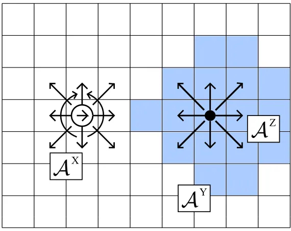
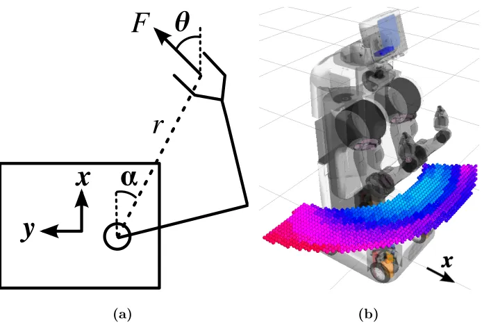
feasible atomic actions. See Figure 4.2 for an example. We define a transition from

the set Tf _{to be the result of a motion primitive applied to a state} _sf_{. Let} _AX _be

the set of motion primitives for X⊂SE(2) and AZ the set of motion primitives for Z⊂SE(3). LetAYbe the set of corresponding motion primitives ofY⊂_Rn_{that make}

the transition in X,Z feasible when the manipulator is grasping an object. AY are defined as relative displacements and are dependent on the starting arm configuration

(47)

X

Y

Z

A

Figure 4.2: Example motion primitives for a mobile manipulator attached to an object. AX

is the set primitives belonging to a mobile base withX= (x, y, θ) constrained to move along

an 8-connected grid or turn in place. AZ is the set belonging to an object with Z= (x, y),

constrained to move on an 8-connected grid. In this case,AY is the set of arm motions which

keep the end-effector on the object during all transitions chosen from the feasible portion of

(48)

freely. In the full-dimensional state-space, we define a motion primitiveaf _{as a 3-tuple}

member of the set Af(Y) = {(aX, aY, aZ)|aX ∈ AX, aZ ∈ AZ, aY applied to Y enables (aX, aZ)}.

4.1.2 Reduced-Dimensional Graph

Let us also define a reduced-dimensional (of dimensionality l) discretized finite state-space Sl _{as the 2-tuple (}_X_,_Z_{). The crux of this work is that we may also represent}

the same mobile manipulation motion planning problem as a graph on the

reduced-dimensional state-space Gl _{= [}_Sl_{, T}l_{], where} _Sl _{is the vertex set and} _Tl _{is the edge set.}

Sl _{is a projection of}_Sf _{onto the lower-dimensional manifold. We define a many-to-one}

mapping γ : Sf → Sl, in which γ((X,Y,Z)) = (X,Z), dropping the manipulator configuration Y. We also define the inverse mapping γ−1 _:_Sl _→ _Sf_{, a one-to-many}

mapping. When an object is grasped by the manipulator,

γ−1((X,Z)) ={(X,Y,Z)|Y∈Y, f(X,Y) = Z}.

Otherwise, when no object is grasped (i.e., the manipulator forms an open chain),

γ−1((X,Z)) = {(X,Y,Z)|Y∈Y}.

There is also a many-to-one mapping ϕ:af →al, whereal is a 2-tuple of the set

Al

(Y) = (aX, aZ)|aX ∈AX, aZ∈AZ,

(49)

We require that edge costs be such that for every pair of states

c(π∗(sf_i, sf_j))≥c(π∗(γ(sf_i), γ(sf_j))) (4.1.2)

The least cost path between any two states in the high-dimensional state-space is

at least the cost of the least-cost path between their images in the low-dimensional

state-space. The transition cost in the high-dimensional graph is

c(π(sf_i, sf_j)) =c1(π(sfi, s f

j)) +c2(π(sfi, s f

j)) (4.1.3)

the sum of two terms that are not interrelated. The first term in Equation 4.1.3 is

also the transition cost function of the lower-dimensional state-space; it is a function

of only X, Z, aX, andaZ. The additive second term is a positive cost as a function of Y and aY.

4.1.3 Algorithm

The overall algorithm is to construct and search the reduced-dimensional graph for

a least-cost path from start to goal, then use that path to reconstruct one of the

corresponding least-cost full-dimensional paths. This decouples the planning for the

manipulator from the planning for the mobile platform. Reconstruction is done by

traversing the path in the lower-dimensional space. Beginning with the first state, aY

(50)

any aY that producessf₂ and satisfies Equation 4.1.1 is selected (either by planning or interpolation of inverse kinematics solutions).

When constructing the reduced-dimensional graph, we must verify the existence

of some aY such that (aX, aY, aZ)∈ Af₍_Y_{) . This check can either be done using an}

inverse kinematics query at plan time, or done in advance as a precomputation (which

is our chosen option). The precomputation is also used eliminate transitions with

self-collisions. When constructing the graph during planning, we also must check

transitions for collisions with the world. It is worth noting that both the high- and

low-dimensional graphs include explicit transitions between grasping and not grasping

an object.

ConstructFullDimPath(π∗(sl

start, slgoal))

setsf_start to initial robot configuration

while sl

n6=slgoal do

compute Yn using IK seeded with Yn−1 setaY=Yn−Yn−1

n=n+ 1

if transition (aX, aY, aZ)∈Af₍_Y_{), then}_continue else compute aY using arm planner

4.1.4 Theoretical Properties

We proceed to show that a graph search on Gl is sound, complete, and optimal. First, for convenience, let us define σ:π(sl

i, slj)→π(s f i, s

f

j), which maps a path in the

lower-dimensional state-space to a set of corresponding paths in the higher-dimensional

(51)

Assumption 4.1.1. We assume that when the manipulator is connected to the object,

the setYof feasible manipulator arm configurations for a given lower-dimensional state

sl

i occupies a path-connected set. For manipulators that do not satisfy this condition,

and thus the feasible configurations are in disconnected sets, we limit ourselves to one

such set.

That is, for any given sl_i = (Xi,Zi), any corresponding feasible Yi can be reached

from any other feasible Yj. Y forms a fully-connected set, though the connections are

not required to be enumerated as part of aY ∈AY. When no object is grasped in the manipulator,Y contains all possible manipulator configurations.

Theorem 4.1.2. Soundness. Any path π(sl_i, sl_j) in Gl can be executed in the full-dimensional space. That is, every π(sl_i, sl_j) corresponds to at least one path π(sf_i, sf_j)

given by σ(π(sl i, slj)).

Proof. As our base case, we know the starting configuration may be mapped to the

full-dimensional space. Assume the mapping σ exists and has produced π(sf_i, sf n),

with j > n > i, terminating in (Xn,Yn,Zn). From the lower-dimensional path, we

have al

n,n+1 = (aXn, aZn) and snl+1 = (Xn+1,Zn+1). By Equation 4.1.1, there exists anaY such that for some starting configuration (Xn,Yj,Zn), there is (aXn, aY, aZn)∈Af(Yj).

However, Yj may not be equal to Yn. Assumption 1 maintains that Yj and Yn are

path connected, so we may transition from Yn to Yj. Then, by definition, applying

(52)

Theorem 4.1.3. Completeness. If there exists a path π(sf_i, sf_j) in the Gf_{, then there}

exists a corresponding path π(sl_i, sl_j) in Gl.

Proof. As our base case, we know the starting configuration may be mapped to the

lower-dimensional space by dropping the Y component. Assume the mapping σ−1

exists and has produced π(sl

i, sln), withj > n > i, terminating in (Xn,Zn). From the

full-dimensional path, we have af_n,n₊₁ = (aX_n, aY_n, aZ_n) and sf_n₊₁ = (Xn+1,Yn+1,Zn+1). The existence of al_n,n₊₁ = (a_nX, aZ_n) is indicated by Equation 4.1.1, because aY_n exists. Applying al

n,n+1 to sln results in the retrieval of the next state sln+1 = (Xn+1,Zn+1). Thus, by induction, the entire corresponding path is given by σ−1₍_π₍_sf

i, s f j)).

Theorem 4.1.4. The cost of a least-cost path from start to goal in Gl _{is a lower}

bound on the cost of a least-cost path in Gf_.

c(π∗(sl_S, sl_G))≤c(π∗(sf_S, sf_G))

Proof. Theorem 2 established that the pathπ_f∗(sf_S, sf_G) can be mapped onto the lower-dimensional state-space Sl_{. Given the restrictions on edge costs in Equation 4.1.2, the}

costs of any transition in Gl are bounded from above by the cost of any transition it maps to in Gf_{. Thus, with all transitions comprising the path bounded from above,}

the cost of a least-cost path from start to goal in Gl _{is a lower bound on the cost of a}

least-cost path in Gf.

(53)

into the higher-dimensional state-space σ(π∗(sl

S, slS)), is also (one of ) the optimal cost

path(s) c(π∗(s_if, sf_j)) in Gf.

Proof. Theorem 4.1.2 established the mapping π(sf_i, sf_j) = σ(π(sl

i, slj)). Because

transition costs are independent of Yand aY, and because the full-dimensional states and transitions are mapped to the reduced-dimensional system by dropping only the

Y andaY terms, the costs remain unchanged. Thus, the lowest cost path in Gl _{is one}

of multiple lowest cost paths in Gf _{due to the multiplicity of the mapping.}

By similar arguments, the paths inGl _{that are}_{-suboptimal (are of at most}_-times

the cost of the least-cost path) are guaranteed to map to-suboptimal paths in Gf. This result is important when using -suboptimal searches like Anytime Repairing A∗, used in the experiments in this chapter.

4.2 Proof of Concept

To demonstrate the benefits of our method, we test extensively in simulation on a

system like that shown in Figures 4.1 and 4.2. We use a mobile base (X⊂SE(2)) with an n-degree-of-freedom planar arm (Y⊂_Rn_{) to move an object around the ground}

plane (the object has no notion of directionality, so Z ⊂ _R2_{). The configuration}

space has been inflated so the robot and object can be represented as points. The

manipulator may attach and detach from the object, switching between open and

(54)

omnidirectional wheels; the planar arms make contact with the cylinder at a height

greater than the height of any world obstacles. Thus, obstacles can collide with the

mobile base and the object being moved, but not with the arms. When the arm makes

contact with the cylinder, we assume it is rigidly attached.

Any state in the full-dimensional state-space is given by

sf = (xr, yr, θr

| {z }

X

, θ1, . . . , θn

| {z }

Y

, xo, yo | {z }

Z

, m

|{z}

W

)

where (xr, yr, θr) ∈X is the mobile base pose, (θ1, . . . , θn) is the joint angles of the

arm, (xo, yo) ∈Z is the cylinder location, and m is a binary value indicating if the

object is attached to the manipulator. A state in the reduced-dimensional state-space

is given by

sl= (xr, yr, θr

| {z }

X

, xo, yo | {z }

Z , m |{z} W )

4.2.1 Implementation

The goal of the planner is to get the object to a desired location on the 2-D grid.

The robot must navigate to the object, attach it to the manipulator, then move it

along the plane to the goal while avoiding obstacles. There is no fixed goal for the

location of the robot base. The heuristic function used to guide the search is the

distance between the robot and object plus the distance between the object location

and the goal. When the robot is connected to the object, only the latter is used. Both

distances are calculated for the entire map during precomputation using 2-D Dijkstra

(55)

The cost function is:

c(al_i,j) = (ccostmap(aX,X) + 1)(cmovement(aX) +cobj(aZ,Z))

where ccostmap(aX,X) represents the maximum cost cell traversed during the transition,

cmovement(aX) the cost associated with moving the robot, and cobj(aZ,Z) the cost

associated with moving the object. The cost is independent of manipulator motion,

satisfying Theorem 4.1.5. The units for the cost functions are seconds; the movement

cost for forward or backwards motion is the distance divided by nominal velocity of

the robot and the cost for turning in place is the angular distance divided by the

nominal angular velocity. The cost for moving the object is similarly a distance divided

by nominal velocity for the object (one could think of it as the speed at which the

object may be moved without tipping). The costmap is unitless with a value of 0 for

unoccupied space and 254 for the obstacles themselves.

A valid configuration of the arm, Y, when not connected to the object is any

configuration not in self-collision. A validYwhen connected to the object must satisfy

the (X,Z) pair. Such pairs are constrained such that the object is at least one arm link length distant from the base, but no more than the total length of the arm. The arm

is assumed to be above the height of the obstacles and so cannot collide with them.

This, coupled with the distance constraint, satisfies the path connectivity requirement

of Y.

The reduced-dimensional lattice is constructed using 12 motion primitives, of which

(56)

for forward and backwards movement. The robot arm is allowed to connect to the

object, but not to disconnect from it. ARA∗ is first run on the reduced-dimensional

state-space representation, initially with suboptimality bound = 5.0 and continued until= 1.0. Full-dimensional paths are generated by populating the arm joint angles using inverse kinematics (using an iterative method, seeded with the previous state’s

joint angles). If the interpolation fails to connect two solutions without self-collision, a

random arm configuration is generated, checked for collision, then used as the seed for

the inverse kinematics call. This method succeeded in generating a full-dimensional

path in all trials.

4.2.2 Results

We tested the graph planner with closed chain abstractions on 100 randomly-generated

maps of size 100 by 100 cells, 10 cm on a side. 50 of these were pseudo-outdoor

environments (random circular obstacles) and 50 were pseudo-indoor environments

(grid obstacles). Robots with planar arms of 3 or 10-links were used; the 3-link arms

had link lengths of 10 cm, while the 10-link arms had link lengths of 4 cm. The graph

planner results were compared against those found by a sampling-based planner,

RRT [57, 64]. The RRT was implemented as two successive searches; the first (S1) was

to bring the robot end effector into contact with the object and the second (S2) to

move the robot end effector, now with object attached, to the goal location. The RRT

Motion Primitives and Planning for Robots with Closed Chain Systems and Changing Topologies

University of Pennsylvania

ScholarlyCommons

Motion Primitives and Planning for Robots with

Closed Chain Systems and Changing Topologies

Steven Robert Gray

Motion Primitives and Planning for Robots with Closed Chain Systems

and Changing Topologies

MOTION PRIMITIVES AND PLANNING FOR ROBOTS WITH

CLOSED CHAIN SYSTEMS AND CHANGING TOPOLOGIES

Steven R. Gray

A DISSERTATION

in

Mechanical Engineering and Applied Mechanics

Presented to the Faculties of the University of Pennsylvania in Partial

Fulfillment of the Requirements for the Degree of Doctor of Philosophy

2013

Vijay Kumar, PhD, Supervisor of Dissertation

Maxim Likhachev, PhD, Co-Supervisor of Dissertation

Jennifer Lukes, PhD, Graduate Group Chairperson

Acknowledgements

Contents

Chapter 1

Introduction

1.1

Background

1.2

Motivation and Contributions

Chapter 2

Literature Review

2.1

Background on Motion Planning

2.2

Planning for Generic Closed-Chain Systems

2.3

Application to Mobile Manipulators

2.4

Motion-Primitive Based Graph Planning

Chapter 3

Preliminaries

3.1

Graph Search

3.1.1

Dijkstra Search

3.1.2

A

Algorithm

3.1.3

Weighted and Anytime Variants

3.2

Lattice State-Space

3.3

Closed Chains

Chapter 4

Planning Framework for Closed

Chains and Systems with

Changing Topologies

4.1

Abstractions for Closed Chain Systems

n-dof

4.1.1

Planning Problem Formulation

A

A

A

4.1.2

Reduced-Dimensional Graph

4.1.3

Algorithm

4.1.4

Theoretical Properties

4.2

Proof of Concept

4.2.1

Implementation

4.2.2

Results