Accuracy Researching of Direction-of-Arrival Estimation Via Music for Circular, Octagonal, Hexagonal And Rectangular Antenna Arrays

ISSN (Online): 2320-9364, ISSN (Print): 2320-9356

www.ijres.org Volume 4 Issue 8 ǁ September. 2016 ǁ PP. 08-15

Accuracy Researching of Direction-of-Arrival Estimation Via

Music for Circular, Octagonal, Hexagonal And Rectangular

Antenna Arrays

Yuri Nechaev

1

, Ilia Peshkov

2

1_{(Information Systems Department/ Voronezh State University, Russia)}

2_{(Radioelectronics And Computer Techniques Department, Elets State University, Russia)}

ABSTRACT:

In this paper circular, octagonal, hexagonal and rectangular antenna arrays for directionof-arrival by using superresolution method MUSIC are considered. The problem of obtaining steering vectors and factor of complicated forms antenna arrays is considered. The steering vectors and array factors are derived by shifting and rotating a reference linear antenna array in space. The root mean square error (RMSE) rate of estimates of MUSIC method in azimuth-evaluation cases are estimated. Additionally the values are estimated in various noise environments and for various geometries of antenna arrays including ranging interelement spacing 0.5λ, 0.75λ, 1.5λ.

Keywords:

circular antenna arrays, direction-of-arrival estimation, MUSIC, super-resolution.

I.

INTRODUCTION

Direction-of-arrival estimation takes a great researching interest in such tasks as direction-finding, sonars and wireless communications and is used to determine radio sources [1]. The antenna arrays shapes used greatly have been studied like uniform linear arrays, rectangular and circular arrays. The main advantage of linear arrays for direction-findings is that has the narrow beam of the radiation pattern, but the scan is only capable for azimuth space. The application demanding as azimuth as elevation scanning makes use of planar arrays [2]. Today the papers devoted to comparative analysis of direction-of-arrival estimation via planar arrays, consider only one or two shapes of arrangements of elements [3, 4, 5, 6, 7, 8, 9, 10, 11, 12, 13]. The main task of this paper is to begin deeply comparing the planar arrays for DOA estimation for the azimuth and elevation scanning.

II.

PROBLEM

FORMULATION

Antenna arrays consist of several antennas aligned and connected in space to form directional pattern. It is possible to scan and steer both the main beam and the nulls of the spatial pattern by changing feeding currents and phases of each antenna element.

The arrays can be built with various geometrical configurations. Linear arrays have the simplest form and aligned along a straight line. Planar arrays have the elements placed on a plane. The planar arrays may be circular, rectangular or arbitrary form of element arrangements. Arrays, whose elements not spaced on a plane or lie on two or more planes, are conformal.

The directional pattern of an array is defined by each element’s patter and their spatial arrangement, amplitude and phase of feeding currents. If each element has the isotropic pattern, then the array’s pattern is overall defined by the geometric form and feeding circuits. The spatial pattern is called an array factor. If each element has non-isotropic form and non-identical, then, according to the pattern multiplication principle, the array’s pattern can be calculated as multiplication of the array factor by the elements’ patterns.

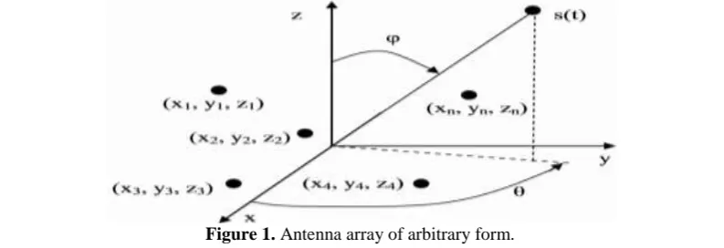
Fig. 1 shows an arbitrary array consisting of N antenna elements randomly arranged in space. Consider a narrowband signal s(t) on carrier frequency ω0 and having angular coordinates θ and ϕ relative to axes x and z

respectively. Note that θ is azimuth coordinate and ϕ - elevation one. The signal can be expressed as [14]:

v(t)) + (ω u(t) = (t)

s cos 0

~ ₍₁₎

where u(t) and v(t) - slowly changing functions of time. The narrowband signal assumes that the amplitude and the phase change slightly small while the waveform transfer from one antenna element to another, that is

 





 





   

  



τ) u(t) ω t τ +v(t)= s(t)= u(t)e t+v(t) (t

s jω0

0 Re Re

cos

~ ₍₂₎

As we can see from fig. 1, the delay depends on relative position of the antenna elements and angular coordinates of the signals. If we take the origin as the reference point and ith element has coordinates (xi, yi, zi) , then the delay τi of the signal at ith element relative to the origin can be expressed as [14]:



x φ θ+y φ θ+z φ



c

=

τ_i 1 _isin cos _isin cos _icos ₍₃₎

where c - speed of light. As the signal is narrowband, then the delay τi produces the phase shift ξi = −τω0, that is

0

ω s(t)e = s(t)e = τ)

s(t jξi jτi ₍₄₎



x φ θ+y φ θ+z φ



c ω =

ξi isin cos isin cos icos

0 ₍₅₎

where λ - wavelength, ω0/c=2π/λ. And now, if the signal at an antenna element is described as x1 , x2 , . . . , xN , then the signal at the array outputs can be described in the vector form as:

 

t =



x

 

t x

 

t x

 

t



T =



ejξ ejξ ejξN



Ts

 

t

N 

 1 2

2 1

x (6)

Denote gi(ω, θ, ϕ) as amplification and phase shift of an antenna element depending on the frequency and signal source direction, then the analytical signal at the array outputs:

 

t =



g(ωθ λ)e g (ωθ λ)e g (ω θ λ)ejξN



Ts

 

t = (ωθ λ)s

 

t

N jξ

jξ

, , ,

, ,

, ,

, 2

2 1

1 a

x  (7)



T



N j N

T j T

j

λ)e θ (ω g λ)e

θ (ω g λ)e θ (ω g = λ) θ

(ω kr1 kr2 kr

a , , ₁ , , ₂ , ,  , , (8)

where



k ,k ,k



=



φ θ φ θ φ



λ π

= x y z sin cos ,sin cos ,cos

2

k - wavenumber, T

n n n T

n =(x ,y ,z )

r - radius-vector pointed

to the nth antenna element. Then the array factor can be written as:



N

= n

T j n(ω θ λ)e

g = AF

0

, , kr

(9)

If a linear antenna array is located the way zero-th element coincides with the origin and oriented along

the x axis, then it is possible to write for the first element r=[1,0,0] and φ θ

λ π =

T

cos sin 2

kr . The same actions

can be done for the case when the antenna elements are located along both y and z. Then the array factor of the linear array can be written:

 



 



N

= n

jnΨ N

= n

z y, x jnk z

y,

x = e

d e = AF

0 0

, (10)

where Ψ=kdcosγ+β, γ - angle between the axis of the linear array and the line from the origin to point of view and can be calculated as dot-product krT.

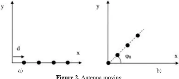
a) b)

Figure 2. Antenna moving

AF e = e e = e + + e + e =

AF jΨ

N

= n

jnΨ jΨ jNΨ Ψ

j jΨ

s 



0

2 ₍₁₁₎

If any kind of antenna array is moved by distance d in the direction γ, then the moved array’s factor is set by the equation (11) [15].

If an antenna array is located at an angle ϕ0 regarding to the x axis as shown in fig. 2(b), then the array factor [15]:



x ,y

 

x φ θ,y φ θ,z φ



=

γ cos sin ,0 sin cos sin cos cos

cos



0



0  (12)



0



0

0sin cos sin sin cos sin cos

cos

cosγ=



φ θ+



φ θ= φ θ



(13)  

 



N 

= n

β + θ φ kd jn r= e

AF

0

0 cos sin

(14)

From equation (14) it is seen, that if the array factor directed along the x axis is represented as AFx (θ,

ϕ) and the antenna array is rotated at angle ϕ0 to the y axis, then the array factor of the rotated array is set [15]:











0





AF

,

AF

r x (15)

In order to calculate a planar array’s factor AFp, it is possible to make several combinations of rotated and moved copies of linear antenna arrays. If linear array’s factor placed along the x is designated as AFx, then by using the properties of the moved linear arrays and combining them, it is possible to get:





y x N

= n

y jk x x

jk x

jk x jk x

p =AF AF

nd e AF = d N e + + d e + d e + AF =

AF



 

  



 _  1

0

1 2

1 (16)

a) b)

c) d)

Figure 3. Antenna array’s geometries

The steering vectors and array factors are necessary to apply direction-finding tasks. However the equation of hexagonal arrays’ factor is very complicated [16], but of octagonal ones is absolutely absent. We can say, that an arbitrary multiple angular antenna array is summation of several moved and rotated linear arrays. Consider building a hexagonal array out of 24 antenna elements. The first side is going to consist of a linear antenna array and located along the x, then its factor will be:



1 0

N

= n

x jk 1

nd e =

Here N = 4 - the number of antenna elements along x-direction. The linear antenna array should be rotated at 60◦ and moved by 4d in order to calculate the second side’s factor. Using the properties (11) and (14), the second side’s factor is set as

 



1 

0 3 / cos sin 4 N = n π θ φ jknd x jk 2 e d e =

AF (18)

The same way, the side 3 is rotated at 120◦ and after that moved by the distance 4d in the direction 30◦ regarding to the x axis.

 





 





_

1   

0 3 / 2 cos sin 4 3 / sin 3 / cos 1 N = n π θ φ jknd y x k j 3 e d π k + π + e =

AF (19)

The similar actions are carried out for the rest of the sides. As a result we get the exagonal antenna array factor (AFHEX):

 





_

     



1 0 4 3 2 4 N n cos sin jknd d sin k k j

e

e

AF

x y    

, (20)

 





_

    



1 0 3 4 4 3 2 5 N n cos sin jknd d sin k j

e

e

AF

y    

(21)    





_

      



1 0 3 5 4 3 3 6 N n cos sin jknd d sin k cos k j

e

e

AF

x  y    

, (22)

 







5 0 p p HEX

AF

AF

₍₂₃₎

So consider using the approach to derive the octagonal array’s factor (AFOCT ) and rectangular one (AFRECT ):















 



























_

_

 













_{ }













_

_

 













_

_

 

 





_

_

4 / 7 3 4 / sin 4 / cos 4 / 6 3 4 / sin 1 4 / cos 4 / 5 3 4 / 2sin 1 3 4 / 2sin 1 4 / cos 4 / 3 3 4 / sin 1 4 / cos 1 4 / 2 3 4 / sin 4 / cos 1 4 / 3 π AF d π k π e + π AF d π + k + π e + π AF d π + e + π AF d π + k + π e = π AF d π + k + π + e + π AF d π k + π + e + π AF d e + AF = AF 1 y x k j 1 y x k j 1 y k j 1 y x k j 1 y x k j 1 y x k j 1 x jk 1 OCT    (24)



/2





cos

 

/2 sin

 

/2



5

 



sin

 

/2



5



3 /3



5 π AF d π e + π AF d π k + π e + π AF d e + AF =

AF jky ₁

1 y x k j 1 x jk 1

RECT (25)

Using AFRECT, AFHEX , AFOCT, we can derive a steering vector to estimate direction-of-arrivals of signals. A steering vector of an octagonal array aoctcan be written as:

                                  _  _ _ _      4 2 1 4 2 2 4 2 3 4 sin 4 cos 1 4 1 4 2 4 3 1 2 , , 1 , , , 1 , , , 1         d N k d k d k d k k j d N k d k d k d jk d N k d k d k OCT x x x y x x x x x x x

x _{e e e e e e e e e e}

e

=   

a

(26)

Steering vectors of hexagonal ahex and rectangular arect can be obtained the same way as aoct from (23) and (25) respectively. Now we can write out signals compex vector of an arbitrary antenna array [2]:

 

t A s(t) n(t)

x  



 

 (27) where x(t) - vector describing signals at output of each antenna element, s(t) - signals vector describing waveforms, n(t) - noise vector, A - matrix of stering vectors corresponding to signals DOA. Spatial correlation matrix can written by the following expression:

H n n n H S S S K k H k

k x E Λ E E Λ E x

R



 

  1 0 )] ( ) ( [

ˆ ₍₂₈₎

where k - time step and K - the number of samples, Es and En - matrices of signal and noise subspaces respectively, Λs and Λn - diagonal matrices of eigenvalues of the signal and noise subspaces respectively. So the spatial spectrum via superresolutional DOA estimation method MUSIC looks like [19]:





1

) ( ) ( ) ,

(  a  E EHa 

N N H MUSIC

P (29)

III.

EXPERIMENTS

Let’s make statistical measurements of MUSIC method in various scenarios. The range of signal-noise ratio (SNR) is from 15 dB up to 0 dB, the number of the averaging samples K of the spatial correlation matrix (28) is 100, the number of the iterations is 500. Root mean square error of bearings of direction-of-arrivals at azimuth and elevation from their true values is fulfilled. Circular, hexagonal, rectangular and octagonal antenna arrays (fig. 3) are compared with each other [17]. All the antennas consist of 24 antenna elements which are evenly spaced along the outer ring of radius r = (12/2π)λ, the distance between adjacent elements are changed in

between 0.5λ, 0.75λ, 1.5λ.

First, consider the case when only one signal arrives at the antennas. Location of the signal will be changed. Herein the signal will be placed on three various levels of elevation angles ϕ: 5◦, 85◦ and in the middle 45◦. After fixing an elevation angle, azimuth coordinates θ will be changed from 0◦ up to 180◦. So that the dependence of RMSE on the signal’s position will be established for the considering arrays. SNR is equal to 5dB in the experiment.

Some conclusions can be made after viewing fig. 4:

1. All the arrays slightly dependent on one signal azimuth location, because the shape of the antenna element arrangements is symmetric.

2. In the case of one signal RMSE of estimates of MUSIC via all the arrays are almost equal to each other. The RMSE of the circular array is a bit less than the others have.

3. If the area of an array gets bigger, RMSE goes down. From fig. 4 it is obviously seen, that ’blue’ curves, corresponding to the interelement spacing equal to 32 λ, have the smallest RMSE and the difference is very high, about 2°.

4. The accuracy of DOA-estimation in azimuth-elevation scenario is highly determined by the source elevation angle. The different elevation positions are marked with different colors and it is clearly seen that ’green’ curves have the highest RMSE, i.e. the worst accuracy is obtained when the signal source is far from the middle elevation angle. The best accuracy can be reached if the signal source is close to ϕ = 45°.

So it can be said that the highest accuracy in DOA-estimation can be reached while using a large aperture antenna array, desirable via circular antenna array and if signal source would be located close to the middle elevation angle, i.e. ϕ = 45◦, independent of azimuth location.

It is much useful studying multiple signals arriving at antenna arrays, because the scenario occurs more frequently in practical situations like indoor, even more in outdoor wireless network or radar applications while several targets bounds electromagnetic wave, etc. Consider two signal sources. Similar to the previous research, the two signals are located successively on the three elevation angles 10◦, 85◦and 45◦. 5◦ was replaced by 10◦ because in the former the performances of MUSIC are very poor. Here we change SNR in the range of 15 dB up to 0 dB. Azimuth positions are 25◦ and 35◦, in the case of ϕ = 10◦, the second source’s position was replaced by

θ = 50◦ also because of the poor resolution.

c) One signal at hexagonal array d) One signal at rectangular array Figure 4. RMSE of one arriving signal at the antenna arrays

a) Two signals at circular array b) Two signals at octagonal array

c) Two signals at hexagonal array d) Two signals at rectangular array Figure 5. RMSE of two arriving signals at the antenna arrays

From curves in fig. 5, we can make some conclusions. First, the two arriving signals produce RMSE of the circular array which is less than others have. RMSE of MUSIC via the octagonal array is slightly higher, the hexagonal array gives highest RMSE, i.e. worse accuracy. The best accuracy can be obtained if the signal source’s location is in the middle of elevation plane, i.e. ϕ = 45◦. Additionally, good accuracy is obtained when the aperture of the antenna arrays gets bigger. If we take an antenna array with interelement distance is 3 2 λ and one with λ 2, smaller RMSE would be obtained via the bigger area antenna, i.e. 3 2 λ. The performances obtained via the rectangular antenna array is not representative because in the multiple signals scenario on the spatial spectrum a lot of false peaks appeared and their identifiability was not possible unlike the circular arrays [18]. But when it was possible and the spatial spectrum was free of false peaks, RMSE of the rectangular array was the smallest.

IV.

CONCLUSIONS

factors of complicated planar arrays has been considered. The approach has been used to obtain both the octagonal, hexagonal, rectangular antenna arrays’ inspirations’ and DOA estimation performances. Based on the expressions, the research of the arrays aiming to directionof-arrival estimation via superresolutional method MUSIC has been fulfilled.

After the simulation, it has been established that the more aperture or area of the antenna arrays the more accuracy of DOA estimation and consequently RMSE decreases. Considering the planar arrays (8-, 6-, 4- side and circular) it has been revealed that the dependence of RMSE on azimuth position is practically absent. Moreover the accuracy and RMSE is highly dependent on an elevation angle. The best accuracy and lowest RMSE are obtained if the signal source (one or more) is located close to the middle of elevation, i.e ϕ = 45◦. If signal(s) are somewhere far away from the middle (up or down), then RMSE increases. The accuracy of DOA estimation via circular or 8-, 6- side arrays are comparable between them, but the circular one has slightly less RMSE values. The rectangular arrays would have the bigger accuracy if they did not have too many false peaks on the spatial spectrum.

V.

ACKNOWLEDGEMENTS

The reported study was funded by RFBR according to the research project No. 16-37-00072.

REFERENCES

[1]. Tuncer, T., Friedlander, B. Classical and Modern Direction-of-Arrival Estimation , Academic Press, 2009, 456 p.

[2]. Godara, L. C. “Applications of antenna arrays to mobile communications,” Proceedings of the IEEE, Vol. 85, No. 8, 1195-1245, 1997.

[3]. Nechaev, Yu., Borisov, D., Peshkov, I. “Beamforming algorithm for circular antenna array immune to multipath propagation and non-stationary interference sources,” Radioelectronics and Communications Systems, Vol. 54, Iss. 11., November 2011.

[4]. Nechaev, Yu. B., Peshkov, I. W. “Accuracy study of superresolution DOA-estimation methods via concentric and circular antenna arrays,” Teoriya i technika radiosvyazi, No. 2., 2016, [in publishing]. [5]. Mahmoud, K. [etc.] “A comparison between circular and hexagonal array geometries for smart antenna

systems using particle swarm optimization.” Progress in Electromagnetics Research, Vol. 72, 7590, 2007. [6]. Gozasht, F., Dadashzadeh, G. R., Nikmehr, S. “A comprehensive performance study of circular and

hexagonal array geometries in the lms algorithm for smart antenna applications,” it Progress in Electromagnetics Research, Vol. 68, 281 296, 2007.

[7]. Dessouky, M., Sharshar, H., Albagory, Y. “Efficient sidelobe reduction technique for small-sized concentric circular arrays,” Progress in Electromagnetics Research, Vol. 65, 187200, 2006.

[8]. Serdar, O. A. “High-Resolution Direction-of-Arrival Estimation via Concentric Circular Arrays,” ISRN Signal Processing, Vol. 2013, Article ID 859590, 8 pages, 2013.

[9]. Ioannides, P., Balanis, C. “Uniform circular and rectangular arrays for adaptive beamforming applications,” IEEE Antennas and Wireless Propagation Letters, Vol. 4, 351354, 2005.

[10]. Kretly, L. C., Cerqueira Jr., A. S., Tavora, A. S. “A hexagonal adaptive antenna array concept for wireless communication applications.” The 13th IEEE International Symposium on Personal, Indoor and Mobile Radio Communications, Vol. 1, 247249, 2002.

[11]. Espandar, M., Bakhshi, H. R. “DOA estimation for rectangular antenna array in multipath fading and MIMO channels,” 2009 International Conference on Future Computer and Communication, Kuala Lumpar, 122-126, 2009.

[12]. Meenakshi, A. V., Punitham, V., Gowri, T. “DOA Estimation for Rectangular Linear Array Antenna in Frequency Non Selective Slow Fading MIMO Channels,” Communications in Computer and Information Science, Volume 203, 12-24, 2011.

[13]. Agatonovi, M. [et ce.], “Efficient neural network approach for 2d doa estimation based on antenna array measurements,” Progress In Electromagnetics Research,Vol. 137, 741758, 2013.

[14]. Trees Van, H. L. Detection, Estimation, and Modulation Theory. Optimum Array Processing, John Wiley & Sons, 2002, 1470.

[15]. Kumar, P. Formulation and Synthesis of Hexagonal Prism Array Using Nature Inspired Algorithm, National Institute of Technology, Rourkela, India, 2014, Master thesis.

[16]. Bird, T. Fundamentals of aperture antennas and arrays, John Wiley & Sons, 2016.

[18]. Nechaev, Yu., Peshkov, I. “Probability of False Peaks Occuring via Circular and Concentric Antenna Arrays DOA Estimation” Telecommunications and Signal Processing (TSP), 2016 39th _{International}

Conference on, Vienna, Austria. [in publishing]