Time Series Analysis of PM10 for Bulandhshahr Industrial Area in NCR using Multiple Linear Regression

e-ISSN: 2278-067X, p-ISSN: 2278-800X, www.ijerd.com

Volume 14, Issue 3 (March Ver. I 2018), PP.56-62

Time Series Analysis of PM10 for Bulandhshahr Industrial Area

in NCR using Multiple Linear Regression

Gaurav Kumar

Associate Professor, Department of Mathematics, NAS College, Meerut Corresponding Author: Gaurav Kumar

Abstract:

Air pollution has become a major problem around National Capital Region (NCR) of India. It has Particulate Matter (PM10) as its one of the constituents. Prediction of air pollutant PM10 can be of help in formulating a policy for air pollution abatement. This paper intends to introduce the reader about air pollution as a problem and also time series analysis of air pollutant PM10 for Bulandhshahr Industrial Area of Ghaziabad city in NCR India using past years data as published by the State Pollution Control Board is conducted using multiple linear regression.

Keywords:

Regression, PM10, Air Pollution, Time Series

--- --- Date of Submission: 25-02-2018 Date of acceptance: 14-03 2018 --- ---

I.

Introduction

Pollution is a pervasive phenomenon of economic growth and development causing harm to society. It refers to the residual flows that arise from anthropogenic sources and enter the environmental systems. The residuals concentration is directly proportional to economic activities and would increase with the rise in activity levels. An economic externality is said to be present when the activities of some economic agents affect the other agents, positively or negatively, which do not have control over them. Air and water pollution, deforestation and land degradation are some of the environmental externalities generated by the various development activities in the economy. The world health organization (WHO) has classified Delhi as one of the most polluted cities in the world along with Mexico City, Seoul and Beijing. The Central Pollution Control Board (CPCB) monitors air quality at various centers in Delhi. The State Pollution Control Board (SPCB) measures air quality at different major cities of the state. Ghaziabad and Noida are two big industrial cities of Uttar Pradesh state of India. These two are part of National Capital Region (NCR) of India and therefore have importance in the development and growth of NCR. These two cities have seen tremendous growth in last two decades. This growth has resulted in the growth of population, vehicles and industrial activities. The growth has resulted in the increase of air pollution beyond the safe level. The major sources of air pollution in these two cities are vehicles and industries. The reduction in the level of different pollutants of air pollution is expected to result in substantial benefits in various sectors of human life. Therefore forecasting of air pollutant becomes an important aspect of policy formulation to tackle problem of air pollution. There are three major air pollutants viz NO2, SO2 and PM10. Time series analysis of PM10 is conducted in this study. A time series is ordering of observation on time scale. This has been used heavily in scientific fields like statistics and signal processing but can also be used in financial forecasting and environment economics. Time series analysis can be done using various methods like Moving Average Method, Artificial Neural Network Method, Trend Reversal Pattern Method, Relative Strength Method, Elliot wave Theory and Regression among others. In this study, Regression method is used to develop time series model for PM10.

II.

Regression Methodology

Multiple linear regression is used in this study. The methodology of the same is given below. Consider the equation -

0 1 1 2 2

....

m m

Y



 



X





X





X





(1)

where 𝑌 is dependent variable, 𝑋1,𝑋2,……,𝑋𝑚 are explanatory (independent) variables, also called regressors or

predictors and 𝜖 denotes the random error term. The above equation represents a linear regression model because the parameters

  

₀

,

₁

,

₂

,....



moccurring in this equation are linear in nature. Let

1 2

(

,

,...,

m

)

2. Error term has zero mean

3. All the predictors

X

_j’s, where j = 1,2,….m and 𝜖 are uncorrelated i.e. we have Cov(𝑋, 𝜖) = 0 4.

X

is nonrandom variable with finite variance

5. None of the predictor variable has perfect correlation with any other predictor variable or with linear combination of the other predictors i.e. there exists no exact linear relationship between the independent variables 𝑋𝑗′𝑠, 𝑗 = 1,2, … 𝑚.

For fixed 𝑋𝑗′𝑠, 𝑗 = 1,2, … 𝑚, the population regression hyperplane is given as conditional mean of 𝑌 for the

given values of 𝑋𝑗′𝑠 i.e.

1 0 1 1 2 2

( |

,...

_m

)

....

_{m m}

E Y X

X



 



X





X





X

(2) as 𝐸 𝜖 = 0. This population hyperplane with parameters

  

₀

,

₁

,

₂

,....



_mis estimated using sample data. From equation (2) –

0

E Y X

( |

1

0,...

X

m

0)









(3)

And the coefficient



_j is given by

1

( |

,...

)

,

1, 2,...,

m j

j

E Y X

X

j

m

X











(4) It is called the jth partial regression coefficient. It represents the change in average value of

Y

when there is increase of one unit in the value of

X

_j.

Once the values of



_j, j = 1,2,….,m, are estimated from sample information, the regression hyperplane is formulated as









0 1 1

...

m m

Y



 



X

 



X

(5)

where 𝑌 is the estimated value of 𝑌 and the





_j′𝑠 represent the estimates of the population parameters. Then the term 𝜖𝑖 = 𝑌𝑖− 𝑌 𝑖, i = 1,2,….n, is the ith residual or deviation from the sample regression hyperplane for n

observations of dependent variable. The population parameters

  

₀

,

₁

,

₂

,....



_mare here estimated using least square method.

2.1 Estimation of the Parameters in the Multiple Regression Model

Suppose n observations are available on the dependent variable Y and let there be m predictors Xj,where j =

1,2,....,m. Let Yi be the ith response level of dependent variable Y and Xij be the ith level of predictor Xj, and then

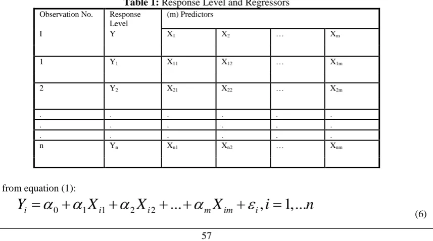
we can represent our sample information consisting of n observations as in below table 1:

Table 1: Response Level and Regressors Observation No. Response

Level

(m) Predictors

I Y X1 X2 … Xm

1 Y1 X11 X12 … X1m

2 Y2 X21 X22 … X2m

. . . .

. . . .

. . . .

n Yn Xn1 Xn2 … Xnm

The principle of least squares is being used to estimate the parameters. Let us choose the parameters



_j’s so that the sum of the squared deviations from the sample regression hyperplane is minimized i.e.



2



2





2



 







0 0 1

1 1 1 1

min

n _i n

(

_{i i}

)

n

(

_i m _{j ij}

)

,

,...,

_m

i

e



i

Y



Y



i

Y







j



X



F

 











(7)

For minima, we must have –







0 1

...

0

m

F

F

F















 









(8)

Here we assume that the second order conditions for minima hold. Then the resulting simultaneous linear equation system can be expressed as -

















1

0 1 1 2 2

2

0 1 1 1 2 1 2 1 1

0

0

...

0

...

...

...

i i i im i

i i m im i

i i i i m i im i i

e

X e

X e

n

X

X

X

Y

X

X

X X

X X

X Y

 























 







 



































2

0 1 1 2 2

...

...

im im i im i m im im i

X

X X

X X

X

X Y

















 









(9)

This is a system of simultaneous linear equations. Solving this system of equations will give the set of parameter estimator



’s. The system given by equation (9) can also be written as:









0

Y

1

X

1 2

X

2

...

m

X

m



 







 



(10)

where

,

ij

,

1,...,

i j i

X

Y

Y

X

j

m

n

n











Substituting equation (10) in remaining m least square normal equations (14), we get:



















1 11 2 12 1 1

1 21 2 22 2 2

1 1 2 2

...

...

...

...

m m y

m m y

m m m mm my

M

M

M

M

M

M

M

M

M

M

M

M

(

)(

)

(

)

(

)

jy ij j i ij i j

jy ij j

il l ij il j l

M

X

X

Y

Y

X Y

n X Y

M

X

X

X

X

X X

n X X





























for j, l = 1,……,m.

This system of equations can be solved for the



’s and then value of



₀can be obtained from equation (10).

2.2 Coefficient of Determination

Let Y = (y1, y2,……,yn) be the observations for output variable and

Y

ˆ



( ,

y y

ˆ ˆ

1 2

,...,

y

ˆ

n

)

be the estimated

value of output variable and

y

be the mean of actual observations of output variable.

The total variability in dependent variable Y can be divided into two parts viz explained variability and unexplained variability.

The explained variability is also called sum of squares due to regression (SSR) and is given by:

2 1

ˆ

(

)

n i i

SSR

y

y









(12)

The unexplained is also called sum of squares due to error (SSE) and is given by:

2 1

ˆ

(

)

n i i

SSE

y

y









(13)

Therefore the total variability (SST) in Y is given by:

SST



SSR SSE



(14)

The coefficient of determination is denoted by R2. It evaluates the goodness of the fitted modeland is given by:

2

SSR

SST

SSE

R

SST

SST







(15)

2

(

)

1

(

)

SSE

R

SST



 

(16)

It is evident that the value of R2 lies between 0 and 1 i.e.

0



R

2



1

.

When SSR is closed to SST then value of R2 will be closed to 1. It means that the regression explains most of the variability in Y and the fitted model is good. When SSE is closed to SST then value of R2 will be closed to 0. It means that regression does not explain much variability in Y and the fitted model is not good. The value of R2 increases whenever an explanatory variable is added to the model. This increase is regardless of the contribution of newly added explanatory variable. Therefore value of R2 may be misleading and so an adjusted value of R2 is defined. It is called adjusted R2 and is given by:

2

/ (

1)

1

/ (

1)

adj

SSE

n m

R

SST

n

 

 



(17)

where m is total number of explanatory variables. Standard error of the estimate is given by:

1

YX

SSE

S

n

m



 

(18)

3. Time Series Analysis

Time series analysis is done using multivariate regression method as described in section 2. The process of forecasting is described as:

An+1 = f(An, An-1,….,A1) (19)

where A1, A2, …., An are the inputs and An+1 is the output.

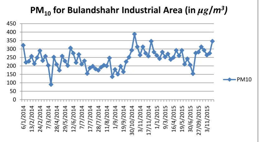
Ghaziabad city being measured at two centers viz Sahibabad Industrial Area and Bulandshahr Industrial Area. This has been above critical level for past few years. Increase in level of PM10 will further deteriorate the air quality of Ghaziabad city. PM10 data from Jan’2014 to Nov’2015 for Bulandshahr Industrial Area has been considered for analysis. Total 69 data points are used to generate the model. Below in figure 1 is a snapshot of data:

Figure 1: Value of PM10 for Bulandshahr Industrial Area

3.2 Regression Model

Linear regression model for Bulandshahr Industrial Area in Ghaziabad city is formulated using IBM SPSS software. Total 69 data points are taken for this centre. These data points are grouped together into 66 groups. Each group contains 4 data points. First 3 data points for PM10 have been considered as input data and 4th in this series has been considered as output data. Again 3 data points, excluding the first data point, are considered as input and next data point as output. The first 3 data points are labeled as PM10_1, PM10_2 and PM10_3, while the output data point is labeled as Observed_PM10. Time series model has been generated as follows:

Table 2: Model Summary

Model R

R Square

Adjusted R Square

Std. Error of the Estimate

Change Statistics Durbi n- Wats

on R

Square Change

F

Change df1 df2

Sig. F Change

1 .548a .300 .267 46.45091 .300 8.876 3 62 .000 1.854

a. Predictors: (Constant), PM10_3, PM10_1, PM10_2

b. Dependent Variable: Observed_PM10

Table 2 shows that the independent variables explain 54.8% of the variability. The result of ANOVA is shown in table 3:

Table 3: ANOVA

Model Sum of Squares df Mean Square F Sig.

1 Regression 57455.320 3 19151.773 8.876 .000b

Residual 133776.619 62 2157.687

Total 191231.939 65

a. Dependent Variable: Observed_PM10

b. Predictors: (Constant), PM10_3, PM10_1, PM10_2

0 50 100 150 200 250 300 350 400 450

6/1/2014 _{13/2/2014 24/2/2014} 7/3/2014 _{28/4/2014 29/5/2014 12/6/2014} 7/7/2014 _{17/7/2014 28/7/2014 11/8/2014} 1/9/2014 _19/9/2014

30/10/2014 3/11/2014 17/11/2014 1/1/2015 9/3/2015 16/4/2015 19/5/2015 30/6/2015 27/09/2015 3/11/2015

PM

₁₀

for Bulandshahr Industrial Area (in

µg

/

m

3

₎

Table 4 shows the t-test results and gives the coefficient of regression equation:

Table 4: Coefficients

Model

Unstandardized Coefficients

Standardized Coefficients

t Sig.

95.0% Confidence Interval for B

B Std. Error Beta

Lower

Bound Upper Bound

1 (Constant) 72.721 33.451 2.174 .034 5.853 139.589

PM10_1 .212 .124 .208 1.707 .093 -.036 .459

PM10_2 .156 .132 .151 1.182 .242 -.108 .421

PM10_3 .336 .127 .326 2.640 .010 .082 .590

Based on table 4, the regression model is given as:

Predicted_PM10 = 72.721 + 0.212 * PM10_1 + 0.156 * PM10_2 + 0.336 * PM10_3 (13)

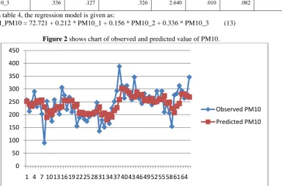
Figure 2 shows chart of observed and predicted value of PM10.

Figure 2: Observed and Predicted Value of PM10

III.

Conclusion

Time series analysis is conducted for prediction of value of PM10 for Bulandhshahr industrial area in NCR of India. Multiple linear regression is used to formulate time series model. The independent variables explained 54.8% of variability which shows that the future value of PM10 can be predicted upto some extent using its past values. There might be some non-linearity in the model. This can be addressed by considering different forms of regression viz log-linear, log-log forms among others. Artificial neural network model can also be built in case of non-linearity.

References

[1] A. C. Goodman and T. G. Thibodeau, “Housing Market Segmentation”, Journal of Housing Economics, vol. 7, no. 2, pp. 121– 143, June, 1998

[2] Berry, J. A. and Lindoff, G., Data Mining Techniques, Wiley Computer Publishing, ISBN 0-471-17980-9, 1997

[3] Calhoum C.A., “Property Valuation Models and House Price Indexes for the Provinces of Thailand: 1992-2000”, Housing Finance International, 17(3): 31-41, 2003

[4] Dasgupta, Purnamita , “Valuing Health Function Approach”, Environment and Development Economics, 9(1): 83-106, 2004 [5] J. E. Zabel and K. A. Kiel, “Estimating the demand for air quality in four US cities,” Land Economics, vol. 76, no. 2, 174–194,

May 2000

[6] Kumar, Gaurav and Sharma R.K., “Air Pollution Evaluation Methods”, International Journal of Engineering Research And Development, Vol 13, Issue 9, 12-17, Sept 2017

[7] Lutkepohl, H, “New Introduction to Multiple Time Series Analysis”, Springer-Verlag, New York, 2005

[8] Murty, M.N. and A. Markandya, “The Cost Benefit Analysis of Cleaning Ganges: Some Emerging Environmental and

0 50 100 150 200 250 300 350 400 450

1 4 7 10131619222528313437404346495255586164

[10] Wei, W.W.S., “Time Series Analysis: Univariate and Multivariate, Methods”, Addison Wesley, New York, 2006