High-performance Computing and Application of Zero-norm

High-performance Computing and Application of

Zero-norm

LiYing Lang

Hebei University of Engineering, Handan,056038，China Email:[email protected]

XueKe Jing

College of Information and Electrical Engineering, Hebei University of Engineering, Handan,056038，China Email:[email protected]

Abstract

--

Whether sparseness can be effectively controlled is one of the key elements to measure the merits of the sparse coding algorithm. One-norm is primarily used in the sparse coding algorithm to control its sparseness currently, as well as by sparse approximation to control the sparseness of sparse coding model, but all these methods have led to slow convergence and low efficiency ultimately. In order to enhance the effectiveness of sparse coding algorithms, this paper selects zero-norm to control sparseness of the sparse coding model, and calculate after continuously extended at the discontinuous point of the model. We propose a highly efficient zero-norm sparse coding algorithm. This paper not only theoretically proves feasibility and efficiency of the algorithms which is capable of effectively controlling model sparseness, but also verifies the theoretical correctness of inference through experiments. These prove the operational efficiency of the algorithm is more efficient and stronger than existing algorithms.

Index Terms--sparse matrix, non-negative sparse coding, sparseness, zero-norm, one-norm

I. INTRODUCTION

Sparse coding theory comes from the studies of optic network, which can simulate the receptive fields of simple cells in the primary visual cortex V1 area, is a method on artificial neural network.

Therefore, many scholars proposed some algorithm models on sparse code, and the method was successfully applied in pattern recognition, data compression, data denoising, etc. [1].

However, sparse coding model can be better used in some areas, but the building and solving of sparse coding model restrict the development of the sparse coding. After Lee and Seung proposed the non-negative matrix factorization [2], some scholars proposed a sparse coding algorithm based on one norm. But this model is difficult to control the sparseness of sparse matrix. Later, Hoyer proposed non-negative sparse coding algorithms (NMFs) [3-4], this algorithm has been widely concerned by people. Although the sparseness of

the algorithm can be controlled effectively by optimal sparse approximation, the algorithm has slow convergence.

This paper attempts use another sparse coding model to solve, the zero norm be used to build model. Although the model is discontinuous function, we can to solve the problem after continuous development in the discontinuity point.The experimental results show that our algorithm can greatly improve convergence rate on the basis of the sparseness of sparse matrix can be controlled effectively.

II. SPARSE CODING MODEL

The standard sparse coding was proposed by Olshausen and Field in 1996. Given a data matrix Vof size M×N, find the sparse matrices Wand H of sizes M

×L and L×N ,where M×N>>(M+N)×L. The sparse model defined as:

min

f

(

W

,

H

)

+

λ

g

(

H

)

(1) Where

_f

₍

_W

_,

_H

₎

is the reconstruction error function between V and WH, and the

_g

₍

_H

₎

is the sparse function of H. The commonly used model of sparse coding defined as:

∑

+

j

i, 0 , 2

2

min

V

WH

_F

_λ

H

_ij

(2)

Where

⎩

⎨

⎧

≠

=

=

₁

0

₀

0

0

ij ij

ij

_H

H

H

, this is the intuitive description of the sparseness of the coefficient matrix. But the standard sparse model is discontinuous function. Mathematical method is more difficult to solve directly. So scholars turn to solve another kind of model, the Zibulevsky[5] proposed a model can write as:

2

min

j i,

, 2

∑

+

i j

F

H

WH

V

_λ

(3) The disadvantage of this model is that it will be equal to the original sparse coding model when the coefficient matrix is very sparse, and the model is not a continuous function, so model to solve difficultly remain unresolved. The model uses one norm to control the sparse degree of

Manuscript received Mar 16, 2011; revised May 30, 2011; accepted June 8, 2011.

the sparse matrix, but the sparse degree is difficulty to control, this model will Lead to the eventual trade-off can not be effectively minimize the reconstruction error and maximization of matrix sparseness.

Hoyer proposed the NMFs[6-7]the model defined as:

H i W i

S

H

spareness

S

W

spareness

t

s

WH

V

=

=

−

)

(

)

(

.

.

min

. . 2 F (4) Although the model can solve the sparse control problem by optimal sparse approximation, it makes slow convergence.

III. ZERO-NORM SPARSE CODING (ZNSC) Standard sparse coding model has the characteristics of discontinuous functions, so the solution is difficulty. We used one norm to describe the sparseness of sparse matrix, which make model is defective in mathematics construction. So in this paper, we try to use zero norm instead of one norm controlling the sparse degree to implement sparse coding algorithm, in order to illustrate the use of zero norm to solve which can better control the sparseness of sparse matrix.

We suppose matrix

⎥

⎦

⎤

⎢

⎣

⎡

=

1

1

1

1

A

and

⎥

⎦

⎤

⎢

⎣

⎡

=

0

0

0

7

B

, so

7

,

4

, 1 , 1

=

=

∑

∑

j i ij j i ij

B

A

. The result is

∑

∑

<

j i ij j i ij

B

A

, 1

, 1 _{, but because the sparseness of}

matrix A less than B, so it is contradict that the one norm of the smaller matrix should obtain great sparseness. However, when we use the zero norm,

1

,

4

, 0 , 0

=

=

∑

∑

j i ij j i ij

B

A

， thus

∑

∑

>

j i ij j i ij

B

A

, 0

, 0 _{, This accurate measure the}

situation of two sparse matrices. If

∑

j i

ij

A

, 0 _>

∑

i j ij

B

, 0 _{, it shows that the number of}

nonzero in the matrix A is greater than that of B. So the sparseness of matrix A is less than that of B. This is consistent with the model

Since the original sparse coding model is discontinuous function, so it is difficulty to solve using the optimization algorithm directly. In this paper, we can to solve the problem after continuous development in the discontinuity point, then linear comparing to complete a sparse matrix solution.

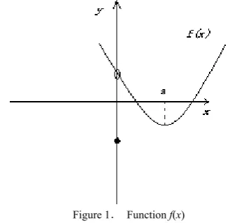
In order to demonstrate this method, we first prove Lemma.

Lemma: if 0

) ( = dx x dg

has a unique solution in the real number field R and

g

(

x

)

has a minimum, then

function

f

(

x

)

=

g

(

x

)

+

c

x

0 _{which obtain the}

minimum in ⎪⎩

⎪ ⎨ ⎧ ≥ + < + ) 0 ( ) ( 0 ) 0 ( ) ( 0 0 0 0 0 0 0 g x c x g g x c x g x ,

Where x0 is the solution of

0

)

(

=

dx

x

dg

and

⎩

⎨

⎧

=

≠

=

0

0

0

1

0

_x

x

x

.

Prove: Let

f

(

x

)

continuous development when

x=0, then set

f

′

(

x

)

=

g

(

x

)

+

c

. Because

)

(

x

g

_{Differentiable and has a unique minimum In the}

real number field R, so

f

′

(

x

)

differentiable and has a unique minimum, the minimum is the solution of

0 ) ( ₌ ′ dx x f d . 0 ) ( ₌ dx x dg

has a unique minimum, set x=

x0.so dx

x dg dx

x f

d ′( )₌ ( )

,then

f

′

(

x

)

obtain the

minimum in

x

0

When

_x

₌

₀

, the value of function

_f

₍

_x

₎

and

)

(

x

f

′

is different. So we can only compare the value of

_f

₍

₀

₎

and

₍

₎

0

x

f

′

, whichever is the minimum of function

_f

₍

_x

₎

of two minimum, we can be seen from Fig 1,the minimum corresponding point is the minima.

If

₀

0

≠

x

, set

0 0 0

0

)

(

)

(

'

x

g

x

c

x

f

=

+

,and

)

0

(

)

0

(

g

f

=

,the conclusion can be obtained. If

0

0

=

x

， no matter

₍

₎

₍

₀

₎

0 0

0

c

x

g

x

g

+

<

or

)

0

(

)

(

x

₀

c

x

_{0 0}

g

g

+

≥

the minimum corresponding

to the point is 0.this satisfy the conclusion of lemma. Proof is completed.

Figure 1． Function f(x)

value of function. Then compare the most value with the value in the break point.

At last, we can obtain the most value.

Theorem

_∀

_k

_∈

_{

₁

_,

₂

_,...,

_L

_}

, set ) 1 ( ] [ T kb ak ab ab W W

F _{= −}

_δ

_δ

,

i

=

k

,then

δ

ik

=

1

,

otherwise

₌

₀

ik

δ

,set kk k k W W H F V W ] [ ] [

HMIN₌ T _T.− .

and 2 T

0

( ) [ ] 2

H kl kl kk kl

f H = H W W +

λ

H +

T T

2 _kl( [ ]_{kq ql}-[ ] )_lk

q k

H W W H V W

≠

∑

,the minimum of the

objective function

₋

₊

_∑

j i j i F

H

WH

V

, , 0 2

2

_λ

will

obtain in ⎩ ⎨ ⎧ ≥ < = ) 0 ( ) HMIN ( 0 ) 0 ( ) HMIN ( HMIN Hnew H l H H l H l l f f f f Prove:

∑

+ − j i j i F H WH V , 0 , 2 2_λ

}

)

)(

{(

_V

_WH

_V

_WH

T

tr

−

−

=

₊

∑

ij

j i H , 0 , 2λ

T T T T

{

2

}

tr VV

HV W

H W WH

=

−

+

+

T T

, ₀ . .

,

2

i j

{

} 2

[

]

j j

i j j

H

tr VV

V W H

λ

=

∑

=

−

∑

+

∑

j

j j

W

WH

H

T T _.

.

+

∑

i j j i

H

, 0 ,

2

_λ

}

,...,

2

,

1

{

N

l

∈

∀

_{,fixed the}

W

_{，then the objective}

function of

H

⋅l _{can be simplified} ：

T T

. . 0

( . )

2[

T

]

2

H l l l l l il

i

f H

=

H W WH

_{⋅ ⋅}

−

V W H

+

_λ

∑

H

=

T

0 ,

[ ] 2 [ T ] 2

ml mn nl lp pl il

m n p i

H W W H − V W H +

λ

H

∑

∑

∑

Further,

∀

k

∈

{

1

,

2

,...,

L

}

， fixed the

W

and

}

{

H

1

,

H

2

,...,

H

k−1

,

H

k+1

,...,

H

L. ，then the objective function of

H

kl_{[8] can be simplified：}

2

0

(

)

[

T

]

2

H kl kl kk kl

f H

=

H W W

+

_λ

H

+

T T

2 kl( [ ]kq ql-[ ] )lk q k

H W W H V W

≠

∑

(5) According to (5) we can know

that

f

H

(

H

k1

),

f

H

(

H

k2

),...

f

H

(

H

kN

)

_{have no}

associated ， and fixed W

and

{

H

1

,

H

2

,...,

H

k−1

,

H

k+1

,...,

H

L.

}

， then the

objective function of

H

k⋅ _{can be simplified ：}

)

(

...

)

(

)

(

)

(

_{k H k1 H k2 H kN}

H

H

f

H

f

H

f

H

f

=

+

+

+

T

T

_]

₎

([

2

}

]

{[

−

_⋅

−

_{⋅ ⋅}

=

H

k

W

T

W

kk

I

H

Tk

W

V

k

F

k

H

H

k

0 .

2

λ

H

_k

（6） Following，we prove the (5) can be solved by the lemma, The key is to proof the

0 )

( ₌

dx x

dg has the only

solution in the real field R. Set

)

]

[

]

[

(

2

]

[

)

(

2

∑

≠

−

+

=

k q lk T ql kq T kl kk T

kl

W

W

H

W

W

H

V

W

H

x

g

then

)

]

[

]

[

(

2

]

[

2

)

(

∑

≠

−

+

=

k q lk T ql kq T kk T

kl

W

W

W

W

H

V

W

H

dx

x

dg

,we can obtain the only solution of

0 ) ( = dx x

dg is

kk T k q ql kq T lk T

W

W

H

W

W

W

V

]

[

]

[

]

[

∑

≠

−

. We can know from the

lemma, the minimum of (5) can be calculated by

continuous development. Because

)

(

),...,

(

),

(

_{k1 H k2 H kN}

H

H

f

H

f

H

f

have no

association, so we can operate continuous development for (6) to obtain the most.

Then operate continuous development for the

function

f

H

(

H

k.

)

_when

H

k⋅

=

0

_.

∀

l

_{, set}

1

0

=

kl

H

, then

H

k. ₀

=

N

_and

T T

. . . .

( ) {[ ] } 2 2([ T ] ) T

H k k kk k k k K

f H′ =H W W I H + λN− W V −F H H

set

f

H

′

(

H

k.

)

=0 to obtain the minimum when

HMIN

₌ kk

T k k W W H F V W ] [ ] [ . . T ₋ ,because among

)

(

),...,

(

),

(

_{k1 H k2 H kN}

H

H

f

H

f

H

f

_{have no}

association, so

∀

l

,according to the lemma we can obtain the minimum of the

f

H

(

H

kl

)

_at

⎩

⎨

⎧

≥

<

)

0

(

)

HMIN

(

0

)

0

(

)

HMIN

(

HMIN

H l H H l H l

f

f

f

f

Proof is completed.

From the above theorem we can know that it is practical to solve sparse coding by zero norm, and the problem of control sparseness can be solved effectively.

In this paper, we use stochastic gradient method to solve the matrix W.ZNSC can be summarized as:

1.Random initialization matrix

_W

₍

₀

₎

,

_H

₍

₀

₎

,

_s

_←

₀

; 2.Repeat the following operation until you meet the conditions so far;

3.W(s+1)←W(s)−μ[W(s)H(s)−V]HT(s);

4.

w

i

←

w

i

/

w

i 2

5.

k

=

1

→

L

(2).Calculate

=

HMIN

kk

L k

k k

k

W

W

s

H

s

H

s

H

s

H

k

F

V

s

W

]

[

)]

(

),

(

),

1

(

,

),

1

(

)[

(

]

)

1

(

[

T

T T T T

1 T

1 T

⋅ ⋅ ⋅

− ⋅

⋅

⋅

−

+

+

+

"

"

(3).

⎩

⎨

⎧

≥

<

=

∀

)

0

(

)

HMIN

(

0

)

0

(

)

HMIN

(

HMIN

H l H

H l H

l kl

f

f

f

f

H

l

6.

s

←

s

+

1

IV. ZNSC ALGORITHM ANALYSIS

In order to illustrate the effectiveness of the algorithm, we compare that with the NMFs and NSC algorithm proposed by Hoyer.

Algorithm: NMF with sparseness constraints [7] 1. Initialize W and H to random positive matrices 2. If sparseness constraints on W apply, then project each column of W to be non-negative, have unchanged

L2 norm, but L1 norm set to achieve desired sparseness 3. If sparseness constraints on H apply, then project each row of H to be non-negative, have unit L2 norm, and

L1 norm set to achieve desired sparseness 4. Iterate

(a) If sparseness constraints on W apply, i. Set W:=W−μW(WH−V)HT

ii. Project each column of W to be non-negative, have unchanged L2 norm, but L1norm set to achieve desired sparseness

Else take standard multiplicative step W:=W

⊗

(VHT₎

∅

_(WHHT ₎

(b) If sparseness constraints on Happly, i. Set H: = H−μHWT_(WH−V)

ii. Project each row of Hto be non-negative, have unit

L2 norm, and L1 norm set to achieve desired sparseness; Else take standard multiplicative step H:= H

⊗

(WT_V)

∅

_(WT_WH)

Above,

_⊗

and

_∅

denote element wise multiplication and division, respectively.

Algorithm: NSC [9]

1.random initialization matrix

0

)

0

(

_≥

W

_,

H

(

0

)

_≥

0

_,

_∀

_i

_，

W

•i

=

W

•i

/

W

•i _{2 ，}

0

←

s

_;

2. Repeat the following operation until you meet the conditions so far;

3.

W

←

W

−

μ

(

WH

−

V

)

H

T 4.

H

←

max{

H

,

0

}

5.

W

←

W

⊗

[

VH

T

]

∅

[

WHH

T

]

6.

∀

i，

W

•i

=

W

•i

/

W

•i 2

7.

s

←

s

+

1

The main difference between ZNSC algorithm and NMFs algorithm are to solve sparse matrix. For ZNSC algorithm, when solve the sparse matrix, each column of

sparse matrix is ordered , and no cycle to determine, however the NMFs algorithm should need to go through the cycle many times and it is not linear, slow convergence rate. Thus, the convergence rate of ZNSC algorithm is superior to the NMFs or NSC algorithm.

V. EXPERIMENT AND ANALYSIS

The convergence speed can not be reflected accurately through comparing the size of each model function value, because of the difference between ZNSC and NMFs algorithm. so the two algorithm can be as the feature extraction algorithm in face recognition, then we can compare their recognition rate by classification algorithm(PSVM)[10], when the recognition rate reaches stability state, the solution of the sparse model can reach convergence state. Therefore we can judge the algorithm’s convergence speed through the time of the recognition rate reaches stability state.

In this paper, we use the ZNSC algorithm, NSC algorithm and NMFs algorithm to do feature extraction on the ORL face database, the proximal support vector machine (PSVM)[11] is used as classifier. The first image of each of the forty kinds of face in ORL face database are chosen respectively to be trained as training samples and we can calculate the basis matrix, where L = 40, L is the column length of coefficient matrix H, and we select the iteration step μ=10-9 in the ZNSC algorithm and NSC algorithm, and λ =100 in the NSC algorithm, the unit of iteration time is second.

■_{A. The Relationship between Regulatory Factors and}

Recognition Rate

Because of using the zero norm, the value of

λ

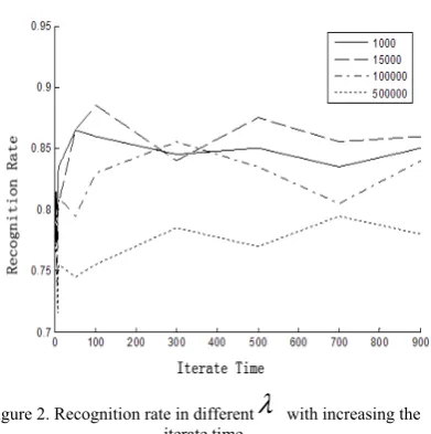
should be determined by the actual situation, in this paper, we choose different

λ

, and observe the change of recognition rate with increasing the iterate time, this result is shown in Fig. 2.

Fig.2 shows that the difference between the recognition rate is not large when the magnitude of

λ

is 103_-104_{,however when the}

λ

_{equals 5×10}5_,the recognition rate begin to decline. From (1), we can know that when the value of

λ

is bigger, the second item becomes major factor, which lead to increased reconstruction error between V and WH. So the value of

λ

should not choose a bigger one.

■_{B. The Relationship between Regulatory Factors and}

Sparseness

The sparseness can be defined as:

1

)

(

0

0

−

−

=

n

x

n

x

sp

(7) Where x may be a scalar, vector, matrix. If x is

scalar ,

x

0 _{show whether x is zero or not. If x is vector}

Figure 2. Recognition rate in different

λ

with increasing the iterate time

Next, observe the change of sparseness with increasing the iterate time. This result is shown in Fig.3 .

The Fig. 3 shows that sparseness is increased with the increase of

λ

, when

λ

is greater than 15000,the sparstiy is more than 0.5. This can meet the general sparse requirements. In addition, the function curve is a straight line basically, this illustrates iteration time has little influence on the sparseness. The sparseness can stabilize in the short period of time.

■_{C. The Efficiency of the Algorithm}

The experimental conditions are that we set

λ

=15000 and other parameters are same as the above experiment. We will compare the recognition rate of three algorithms. The result is shown in Fig. 4.

From Fig.4 we can see that three algorithm’s recognition isn't monotone rising with the increase of iterative time, because initial matrix is selected randomly when iteration is operated every time, at last which lead to the result of convergence is different. Overall, the recognition rate can reach up to 85% within tens of seconds, and recognition rate shows a steady trend with the increase of iterative time. This shows that ZNSC algorithm can achieve a stable recognition rate in a few seconds. But the recognition rate is not good by NMFs algorithm. we can see that the recognition rate only reaches 80 percent when the iterative time in 300 seconds, this shows that its convergence speed is relatively slow.

Although the iteration time of NSC is shorter than that of NMFs, it is also more time-consuming than ZNSC algorithms.

The above has stated that ZNSC algorithm is better than NMFs on the recognition rate, and ZNSC algorithm can reach the desired results in a short time. We can see from Fig.3 the ZNSC algorithm’s iteration reach the stable value at beginning, it shows that the algorithm of this paper reached the expected sparse degree at first, that is to say the algorithm in this paper indeed achieve the ideal convergence state in a shorter time.

Figure 3. Sparseness of the sparse matrix in different

λ

with increasing the iterate time

Figure 4. Recognition rate of the three algorithms with different iterate time

VI. CONCLUSION

This paper can solve controlling problem of sparse degrees effectively by using zero norm measure the sparseness of sparseness matrix to solve the problem of sparse coding. Firstly this model just do one addition, subtraction, multiplication and division method in solving each column of sparse matrix, then get the results by doing a judgment for each value of column vector in parallel, but all the columns of the matrix is linear, no cycle computing. This shows that this algorithm is more effective in speed to solve sparse matrix comparing with NMFs algorithm, and ideal sparse matrix can be taken in a short period.

REFERENCES

[1] Garrigues, P., Olshausen, B.. Learning horizontal connections in a sparse coding model of natural images[J]. Advances in Neural Information Processing Systems, 2008,pp. 505-512.

[2] Ouhsain M,Hamza A B.Image watermarking scheme us-ing nonnegative matrix factorization and wavelet transform.Expert Systems with Applications, pp.2123-2129,2009.

[3] Fevotte, N. Bertin, and J. L. Durrieu. Nonnegative matrix factorization with the itakurasaito divergence: With application to music analysis. Neural Computation, PP.793–830,2009.

[4] J Mairal, F Bach, J Ponce,G Sapiro.Online Learning for Matrix Factorization and Sparse Coding.Journal of Machine Learning Research,2010,pp.19-60.

[5] Zibulevsky M and Pearlmutter B A. Blind source separation by sparse decomposition in a signal dictionary. Neural computation,2001,pp.863-882.

[6] Hoyer P O．Modeling receptive fields with non-negative sparse coding[C]IEEE Workshop on Neural Networks for Signal Processing,Toulouse，France，2003, pp. 547-552. [7] Patrik O.Hoyer．Non-negative Matrix Factorization with Sparseness Constrains[J]．Journal of Machine Learning Research, 2004,pp.1457-1469.

[8] LI Le, ZHANG Yu-Jin．a Stable and Efficient Algorithm for Nonnegative Sparse Coding[J]．Acat Automatica Sinica, 2009,pp.1257-1271.

[9]Hoyer P O. Non-negative sparse coding[C].//IEEE Workshop on Neural Networks for Signal Processing,Valais，Switzerland，2002,pp.557-565.

[10]N. Saravanan , K.I. Ramachandran.A case study on classification of features by fast single-shot multiclass PSVM using Morlet wavelet for fault diagnosis of spur bevel gear box,India,pp.10854-10862,2009.

[11]Liu Y, Zhang H H, Park C, et al. Support vector machines with adap tive Lq penalty,J.Comput Statist and Data Anal, pp. 6380-6394, 2007.

LiYing Lang HeBei Province, China.

Birthdate: September, 1974.is Optical Engineering Doctor, graduated from Tianjin University of Optical Engineering. And research interests on Face recognition and image processing.

She is a associate professor of Dept. School of Information and Electrical Engineering, Hebei University of Engineering

XueKe Jing HeBei Province, China. is