Object Tracking via Tensor Kernel Space Projection

Object Tracking via Tensor Kernel Space

Projection

Jiashu Dai

College of Computer Science and Technology, Harbin Engineering University, Harbin, China Email: [email protected]

Tingquan Denga Tianzhen Donga Kejia Yib

a. Laboratory of Fuzzy Information Analysis and Intelligent Recognition, Harbin Engineering University, Harbin, China b. Science and Technology on Underwater Acoustic Antagonizing Laboratory, Systems Engineering Research Institute

of CSSC, Beijing, China

Email: {tq_deng, tianzhen.d, yikejia2007}@163.com

Abstract—Although there has been significant progress in the past decade, object tracking under complex environment is still a very challenging task, due to the irregular changes in object appearance. To alleviate these problems, this research developed an object tracking algorithm via tensor kernel space projection. In the initial stage of tracking, a template matching algorithm was used to obtain a priori images of the appearance of the object. The steps taken were as follows: define the tensor kernel function based on a multi-linear singular value decomposition, view the object appearance color image as tensor data, calculate the kernel matrix for the priori appearance image samples, use KPCA to obtain the projection matrix of the image samples in kernel space, and finally, obtain an optimal estimate of the object state through Bayesian sequence interference. Meanwhile, the projection matrix in kernel space was updated on-line. Experiments on two real video surveillance sequences were conducted to evaluate the proposed algorithm against two classical tracking algorithms both qualitatively and quantitatively. Experimental results demonstrate that the proposed algorithm is robust in handing occlusion and object scale changes.

Index Terms—object tracking, tensor kernel, SVD, kernel pace, projection

I. INTRODUCTION

Object tracking as an important research area in computer vision and pattern recognition, has many applications, such as: object recognition, video surveillance, traffic monitoring, human-computer interaction, video compression, weapon automatic tracking, etc. [1-3].

The chief challenge in object tracking is how to adapt to appearance variability in the object. The appearance variability includes the effects of: camera motion, camera viewpoint changes, illumination change, pose variation, shape deformation and occlusions [4]. To solve this problem, there are two types of methods based on different appearance models: generative and discriminative methods.

Generative methods model appearance of targets use gray value or other features, and predict the target state by find the image patch most similar to the target. The classical mean-shift [5-6] tracking method using the kernel function forms a weighted model of the color histogram, and defining the similarity measure by its Bhattacharyya coefficient, seeks the most similar region to the reference template by a first-order gradient descent algorithm. The CBWH tracker [7] transforms only the object model but not the object candidate model. Ross [4] uses an incremental sub-space model combined with a particle filter to adapt to appearance changes. Gao [8] uses a Mexican hat wavelet to change the mean-shift tracking kernel and embedded a discrete Kalman filter to achieve satisfactory tracking. The

l

1-tracker [9] uses a

visual tracking problem as a sparse approximation, obtains sparse representation by solving

l

1 regularisation,

and finally finds the minimum reconstruction error region. Gao [10] fused multi-feature weights through DS evidence theory and combined with a particle filter achieves better results when considering the particle degeneration phenomenon.

Discriminative methods formulate object tracking as a binary classification problem for separates the target from the background. The Support Vector Tracking [11] integrates SVM into optical flow classifier for object tracking. Avidan [12] combined weak classifiers into a strong classifier to distinguish the object with background. The online boosting tracker [13] selects features using boosting classifier. The MIL tracker [14] using Multiple Instance Learning to overcome slight inaccuracies in labeled training examples can cause drift, the samples are considered within positive and negative bags.

The authors proposed an algorithm that uses tensor kernel space projection for object tracking to estimate the object state in real-world scenarios. For the purpose of highlighting the real differences between color images, a tensor kernel based on multi-linear singular value decomposition was defined. The Bayesian sequence interference framework was combined therewith to project the observe image samples in kernel space using a kernel matrix. Experimental results showed that the

Supported by the Natural Science Foundation of Inner-Mongolia Autonomous Region China under grant 2012M0931.

proposed algorithm could achieve object tracking in real-world and occlusion environments, it was also adaptive to object scale changes.

II. TENSOR KERNEL BASED ON MULTI-LINEAR SINGULAR

VALUE DECOMPOSITION

A. Tensor Algebra

A tensor can be seen as a multi-order array which exists in multiple vector space, meanwhile, tensor algebra forms the mathematical basis of the multi-linear analysis [15]. A scalar is a zero-order tensor, a vector is a first-order tensor and a matrix is a second-first-order tensor. It is obviously that a color image is a third-order tensor. An N -order tensor can be denoted by _X∈_RI1× × ×I2"IN _{, the}

element of X is

1, , ,n ,N i i i

x " " , where1≤ ≤in In.

Definition 1: The n-mode unfolding matrix of a tensor dataX is denoted as

1 1 1

( )

( )

n n n N

I I I I I n

− +

× × × × × ×

∈

" "

X

R

(1)

The element

1, , ,n ,N i i i

x " " of X in X( )n at in-th row and at

1 2 1 1 1 1 1 2

[(i_n+ −1)I_n+ "I I_N "I_n− + +" (i_N−1)I"I_n− +(i −1)I

1 1]

n n

I ₋ + i₋

" " -th column.

Definition 2: The n-mode product of a tensor data

1 2 N I× × ×I I

∈ "

X R and a matrix _U∈RJn×In _denoted

as I1 In1 Jn In1 IN n

− +

× × × × ×

× ∈ " "

X U R .The element ofX×nUis

(

)

1 2 N

1 n1n n1 N n n

n

n _{i i j i i} i i i j i i

x

u

− +

×

_{" "}

=

∑

"

X

U

(2)

Definition 3: The inner product of two tensors

1 2 N

, ∈ I× × ×I "I

X Y R denoted as

1 N 1 N

1 2

,

n n

N

i i i i i i i i i

x

y

=

∑∑ ∑

"

" " " "

X Y

(3)

B. Tensor Kernel Based on Multi-linear Singular Value Decomposition

Tensor data can retain the original spatial structure of an object. Viewing the object color image as tensor data can help us exploit the intrinsic geometric relationships of object classes. The object image data belong to the same class reside in a low-dimensional manifold embedded in high-dimensional vector space.

The purpose of the kernel method is to identify and learn the relationship in a data set.

Fig.1 The schematic diagram of tensor kernel based on multi-linear SVD.

The original data can be embedded in high-dimensional feature space through a nonlinear mapping ϕ . The

traditional kernel function k x y( , ) for vector data is

known as: RN×RN →R and

X

Y

(1) X

(2) X

(3) X

(1) Y

(2) Y

(3) Y

1( , )

k X Y

2( , )

k X Y

3( , )

k X Y

( , )

k X Y

(1)

SVD(X )

(2)

SVD(X )

(3)

SVD(X )

(1)

SVD(Y )

(2)

SVD(Y )

(3)

satisfied k( , )X Y = ϕ(X), ( )ϕY , so the kernel

function k x y( , ) for tensor data must obey the rule:

1 2 N 1 2 N

RI× × ×I "I ×RI× × ×I "I →R .

Kernel methods for non-linear models have proven successful in many computer vision fields[16]. So it is feasible to improve the discriminatory power of supervised tensor-based models using a tensor kernel. The most recent tensor-based techniques are based on matrix unfolding. The multi-linear singular value decomposition of tensor data X can be reduced to the SVD of X_{( )n} , whereX_{( )n} is the matrix unfolding of X ,

N

n≤I ,

( ) X_{( )} X_{( )} X_{( )}

X

n n n

T n

=

U

Σ

V

(4)

whereUX( )n ,ΣX( )n , X( )n T

V are the three components of this

SVD, and can be sated in block-partitioned form,

(

)

( ) ( ) ( )

1 2

X_n X_n X_n

U

=

U

U

(5)

( ) ( ) 1

0

0

0

X X n n

⎛

Σ

⎞

Σ

= ⎜

_⎜

⎟

_⎟

⎝

⎠

(6) ( ) ( ) ( ) 1 2 X X X n n n T T T

V

V

V

⎛

⎞

⎜

⎟

=

⎜

⎟

⎝

⎠

(7)

Definition 4: Given a datasetX :X X₁, ₂,",X_m∈X , the kernel matrix of this set is an N×NmatrixK, and the elementk_ijis

(

,

)

ij i j

k

=

k

X X

(8)

A simple template matching object tracking method used in the first mframe images, then we can get the prior acquisition object sample tensor dataset{X X1, 2,",Xm}.

Because

k

_ij

≥

0

, the kernel matrixK is non-negative, and positive semi-definite.

( , )

i

k X Y correspond to the kernel function in mode iof the two tensors, and can be calculated by:

( ) ( ) ( ) ( )

1 1 1 1

2

( , )

exp

2

i i i i

T T

i

V

V

V V

k

σ

⎛

₋

⎞

⎜

⎟

=

_⎜

−

_⎟

⎜

⎟

⎝

⎠

X X Y Y

X Y

(9)

Where

σ

indicates an appropriate bandwidth.

Then the kernel function between tensors is defined as:

1 2 3

( , )

( , ) ( , ) ( , )

k

X Y

=

k

X Y

k

X Y

k

X Y

(10) The kernel function of colour image tensor data is showed as Figure1.

III.TENSOR KERNEL SPACE PROJECTION

Principle component analysis can only handle the linear information in a dataset, a kernel trick may be used in kernel space to distinguish object and background [17].

Given a training datasetα α1, 2,",αm, using kernel

mapping ϕ projecting them into kernel space, we getϕ α ϕ α( 1), ( 2),", (ϕ αm) , Let ℵ =[α α1, 2,",αm] and

1 2

( ) [ ( ), ( ), , ( _m)]

ϕℵ = ϕ α ϕ α "ϕ α . Projecting ϕ α( _i) in kernel space along projection directionp,

(

)

T

i

p

i

β

=

ϕ α

(11) The total dispersion of the projected training dataset is

1 1

1

(

)(

)

1

( (

)

)( (

)

)

m T i i i m T T i i i T

D

m

p

p

m

p Sp

β β β β

ϕ α

α ϕ α

α

= =

=

−

−

⎡

⎤

=

_⎢

−

−

_⎥

⎣

⎦

=

∑

∑

(12)

Where 1 ( ) m i i m ϕ ϕ α = ⎡ ⎤

= ⎢_⎣

∑

⎥_⎦ is the mean value of the

dataset in kernel space.

The purpose of this kernel space projection is to find the optimal projection direction pby maximizing the total dispersion of the projected training datasetD. Thus,

( )

arg max

T

p

J p

=

p Sp

(13)

To maximize the objective function, we need to find the Eigen-value decomposition toS.

1 1

1

( (

)

) ( (

)

)

1

=

( (

)

)

( (

)

)

n T i i i m T i i i

p

Sp

p

m

p

m

λ

ϕ α

ϕ ϕ α

ϕ

ϕ α

ϕ

ϕ α

ϕ

= =

=

=

−

−

⎡

₋

⎤

₋

⎢

⎥

⎣

⎦

∑

∑

(14) Herepcan be regarded as the feature vector ofS. It can also be seen that the projection directionpis the linear composition of ( (ϕ α_i)−ϕ), Namely that

[

1 2

]

( )

( (

)

), ( (

)

),

, ( (

_m

)

)

ψ

ℵ =

ϕ α

−

ϕ ϕ α

−

ϕ

"

ϕ α

−

ϕ

(15) That is 1

( (

)

)

( )

m i i i

p

c

ϕ α

ϕ

ψ

C

=

=

∑

−

= ℵ

(16)

Where

[

1, 2, ,

]

T l

C= c c " c is the matrix which comprising the linear combination coefficients. Now, solving for the optimal projection direction was transformed into a problem whereby solving the combination coefficient matrix was required, the objective function became:

2

1

( )

arg max

T

( )

T

( )

C

J C

C

C

m

⎡

ψ

ψ

⎤

=

_⎣

ℵ

ℵ

_⎦

(17)

LetAmis am m× matrix with all entries equal to1m,

( )T ( )

m m m m

K

= −

K

A K

−

KA

+

A KA

(18)

Eigen-value decomposition to

S

,

(

)

Sp

=

λ

m p

(19)

Then

( )

T

S

( )

C

(

m KC

)

ψ

ℵ

ψ

ℵ =

λ

(20)

(

)

KC

=

λ

m C

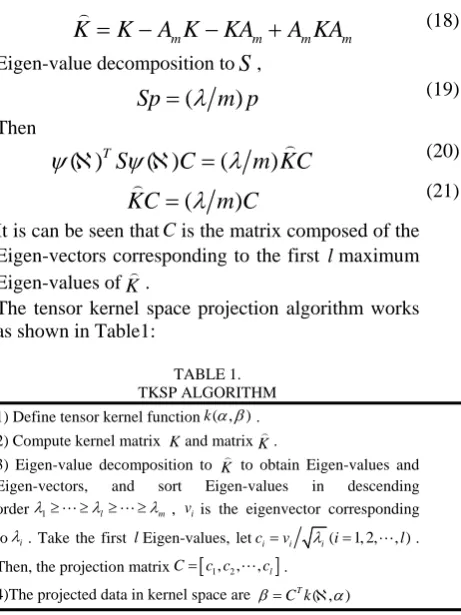
(21)

It is can be seen thatCis the matrix composed of the Eigen-vectors corresponding to the first lmaximum Eigen-values ofK .

The tensor kernel space projection algorithm works as shown in Table1:

TABLE 1. TKSP ALGORITHM 1) Define tensor kernel function ( , )kα β . 2) Compute kernel matrix Kand matrixK.

3) Eigen-value decomposition to K to obtain Eigen-values and Eigen-vectors, and sort Eigen-values in descending orderλ1≥"≥λl≥"≥λm, viis the eigenvector corresponding toλi. Take the first lEigen-values, letci=vi λi(i=1, 2,", )l . Then, the projection matrixC=[c c1, 2,",cl].

4)The projected data in kernel space are T ( , )

C k

β= ℵα

IV.BAYESIAN SEQUENCE INTERFERENCE FRAMEWORK

FOR OBJECT TRACKING

A. Bayesian Sequence Interference

In the problem of object tracking, the object state in the current frame only related to the object state in the prior frame. Define o_t as the state variables of the object at time t. Letot =( ,x y w ht t, t, )t , wherex y w ht, t, t, t denotes

the center coordinate, the width and height of the tracking rectangle.

Given a set of targetsZ_t =

{

z z₁, ₂,",z_t

}

, the objective of object tracking is to obtain the optimal estimate value of the hidden state variablesot. According to Bayesian

theorem, it can be obtained in a similar fashion as that of the object state:

(

t t

)

(

t t

) (

t t 1

) (

t 1 t 1

)

t 1

P o Z

∝

P z o

∫

P o o

₋

P o

₋

Z

₋

do

₋

(22)

Where

P o o

(

_{t t−1}

)

refers to the state transition model

and

P z o

(

_{t t}

)

refers to the observation model. It can be

seen that the observation model

P z o

(

_{t t}

)

determine the tracking results.

State transition model: This was used to model the object motion between consecutive frames. Because of the irregular movement of object, the stateot is modeled by

independent Gaussian distribution around its counterpart in stateot−1. Described as

(

t t 1

)

(

t

;

t 1

,

)

P o o

₋

=

N o o

₋

Δ

(23)

Where Δ means the diagonal covariance matrix ofx y w ht, t, t, t, and the element is

2 2 2 2

, , ,

x y w h

σ σ σ σ . Point to Gaussian distribution, N particles can be randomly generated. According to the particle can obtain multiple states

{

o iti, =1, 2,",N

}

. During the computing process, with the increase in the number of particles, the a posteriori probability estimate was more accurate, but at the same time, the computational efficiency was low, so a balance was sought between these factors.

Observation model: this was used to measure the similarity between the appearance observation and the object appearance model. Given a drawn particle state i

t

o and a cropped version of the corresponding image

patch i t

z from the frame image It. The probability of an

image patch being generated from the kernel space is inversely proportional to the difference between image patch and the appearance model, and could be calculated between the negative exponential distance of the projected data and the center of dataset

{

}

(

_ti _t

)

exp

_ti

F

p z o

=

−

s

−

s

σ

(24)

Where

σ

indicates an adjustment factor, •_F is the Frobenius norm, sti =C k X zT ( , ti), ( , )

T

s =C k X x , C is the projection matrix in kernel space, and xis the center of dataset in kernel space.

The state oticorresponding to the maximum ( ) i t t

p z o is the optimal object state at time t.

B. Projection Matrix Online Update

Along with the movement of the object in scenarios, the object appearance also changed. The projection matrix in kernel space must be updated on-line so that at time t, we have obtained the former t - 1 time object states. When t - 1 is the times used as initial training dataset numbers, we recalculated the projection matrix in kernel space using the newly acquired t - 1 object tensor data points.

Fig.2 The flow chart of the proposed visual tracking algorithm.

V.COMPARATIVE EXPERIMENTS AND ANALYSIS

All the experiments were carried out in the MATLAB® 2010a environment running on a Pentium® Dual-Core E5200 processor with a clock-speed of 2.50 GHz.

In these experiments, we use Portuguese shopping center video monitoring data to test. The video frame image size was 388 284 3× × , and the experimental data were compared with classical CBWH, and MIL, tracking algorithms. The CBWH tracking algorithm select 16×16×16 bin histogram. In MIL tracking algorithm, the feature pool is 250, weak classifiers number is 50 and the learning rate is 0.85. The variance of Gaussian distribution is [2, 2, 0.5, 0.5] in the proposed tracking algorithm. In the initial frame, the object tracking rectangle was manually/artificially marked, and a

template matching tracking algorithm was used to get the previous twenty frame object states.

A. Expeiment A

We first selected scale changes in an environment of complex surveillance scenario, meanwhile the movement of object was irregular. The object was walking toward the camera. The length of this video was 200 frames.

The tracking results of experiment A are shown as Figure 3. It can be seen from the pictures that when a similar object appeared around the target, the CBWH and MIL tracking algorithms cannot achieve well tracking; our tracking algorithm could adapt thereto. In the tracking progress, the size of the object changed from 28 × 79 to 44 × 111.

CBWH tracking algorithm

MIL tracking algorithm

Proposed tracking algorithm

The 1st frame The 73rd frame The 96th frame The 114th frame Initial stage I:

Automatic detection or artificial marked

object initial state

Initial stage II: Obtain prior object states

through template matching.

Learning stage I: Calculate tensor kernel of prior object

tensor data. Learning stage II: Tensor kernel space

projection.

Tracking stage I: Bayesian sequence interference tracking

Tracking stage II: Update kernel space

CBWH tracking algorithm

MIL tracking algorithm

Proposed tracking algorithm

The 157th frame The 172nd frame The 184thframe The 200th frame

Fig.3 The tracking results of experiment A.

B. Expeiment B

The second video had scale changes and occlusion in the surveillance scenarios studied. The object was walking away from the camera. The object was walking away from the camera. The length of this video was 300 frames.

The tracking results from experiment B are shown in Figure 4. It can be seen from the pictures that when the

object was almost occluded by other moving objects, the CBWH and MIL tracking algorithms suffered interference from the other objects, and could not have tracked the target. Our tracking algorithm overcame the problem of occlusion and tracked the target.

In the tracking progress, the size of object changed from 39× 112 to 21× 64.

CBWH tracking algorithm

MIL tracking algorithm

Proposed tracking algorithm

The 1st frame The 80th frame The 140th frame The 186th frame

MIL tracking algorithm

Proposed tracking algorithm

The 194th frame The 200thframe The 260thframe The 300th frame

Fig.4 The tracking results of experiment B.

C. The Evaluation of Tracking

To quantitatively compare the experimental results of the tracking algorithms, we used two metrics to describe it: Tracking errors and Tracking correct ratio. We initially hand-labelled the object state in each experimental scenario.

The error in X-axis e_xis

e

x g

e = x −x

(25) Where x xe, gare the X-axis coordinates of the center

of the experiment tracking rectangle and the ground truth rectangle.

The error in Y-axis eyis

e

y g

e = y −y

(26) Where y ye, gare the Y-axis coordinates of the center

of the experiment tracking rectangle and the ground truth rectangle.

The error in center coordinate ecis

2 2

e e

( ) ( )

c g g

e = x −x + y −y

(27) The error in experiment A and B are shown as Table 2 and 3. The data in bold refer to optimal results.

TABLE 2

THE ERRORS OF EXPERIMENT A

Items(pixels) x-errors y-errors c-errors Proposed Method 1.7145 2.3905 3.2788

CBWH 4.0725 15.6325 16.9349 MIL 4.2025 5.0400 6.8776

TABLE 3

THE ERRORS OF EXPERIMENT B

Items(pixels) x-errors y-errors c-errors Proposed Method 1.8276 2.4318 3.2209

CBWH 7.0183 19.1450 21.0142 MIL 12.7800 19.4817 23.5559

The tracking correct ratio ris

e

e

( )

( )

g

g

area R R r

area R R

∩ =

∪ (28) Where R_eis the experiment tracking rectangle, R_g is the ground truth rectangle, area()means the area of the region. It was thought that if the tracking correctly ratio was greater than 0.5, the tracking in this frame was

successful. The tracking correctly ratios in two scenarios are shown as Figures 5 and 6. The red line indicates the results of the proposed tracking algorithm, the green line indicates the CBWH tracking algorithm and the blue line indicates the MIL tracking algorithm. It can be seen that our proposed tracking algorithm had better results than the other two tracking algorithms. Also, the tracking correctly ratio of our algorithm was almost always greater than 0.5, implying that the algorithm was successful.

Fig.5 The tracking correct ratio in experiment A.

Fig.6 The tracking correct ratio in experiment B. Proposed CBWH MIL

VI.CONCLUSION

In this work, we proposed the use of a tensor kernel space projection for object tracking in video surveillance scenarios. Considering the spatial structure of the object image, we defined a tensor kernel function based on multi-linear singular value decomposition. We projected the object image tensor data into kernel space, and combined this with a Bayesian sequence interference tracking framework to achieve object tracking. To adapt to the object appearance changes, we updated the projection matrix on-line and also analyzed the performance of our proposed tracking algorithm in an assessment against challenging real-world video surveillance scenarios and compared the output with two classical tracking algorithms. The experimental results demonstrated the accuracy and robustness of the proposed tracking algorithm.

REFERENCES

[1] A. Yilmaz, O. Javed and M. Shah, "Object tracking: a survey," ACM Computing Surveys, vol. 38, pp. 1-45, 2006. [2] H. Yang, L. Shao, F.Zheng, L. Wang and Z. Song, "Recent

advances and trends in visual tracking: a review,"

Neurocomputing, vol. 74, pp. 3823-3831, 2011

[3] Z. Feng, B. Yang, Y. Zheng, H. Tang and Y. Li, "Initialization of 3D human hand model and its applications in human hand tracking," Journal of Computers, vol. 7, pp. 419-426, February 2012.

[4] D.A. Ross, J. Lim, R. Lin and M. Yang, "Incremental learning for robust visual tracking," International Journal of Computer Vision, vol. 77, pp. 125-141, 2008.

[5] D. Comaniciu, V. Ramesh and P. Meer, "Kernel-based object tracking," IEEE Transactions on Pattern Analysis and Machine Intelligence, vol. 25, pp. 564-577, 2003. [6] H. Zhou, Y. Yuan and C. shi, "Object tracking using sift

features and mean shift," Computer Vision and Image Understanding, vol. 113, pp. 345-352, 2009.

[7] J. Ning, L. Zhang, D. Zhang and C. Wu, "Robust mean shift tracking with corrected background-weighted histogram," Iet Computer Vision, vol. 6, pp. 62-69, 2012. [8] T. Gao, Z. Yao, P. Wang, C. Wang and J. Yang,

"Automatic Stable Scene based Moving multi-target detection and tracking," Journal of Computers, vol. 16, pp. 2647-2655, Decemble 2011.

[9] X. Mei and H. Ling, "Robust visual tracking and vehicle classification via sparse representation," IEEE Transactions on Pattern Analysis and Machine Intelligence,

vol. 33, pp. 2259-2272, 2011.

[10]J. Gao, W. Li, D. wu, "Multi-feature fusion tracking based on a new particle filter," Journal of Computers, vol. 7, pp. 2939-2947, December 2012.

[11]S. Avidan, "Support vector tracking," IEEE Transactions on Pattern Analysis and Machine Intelligence, vol. 26, pp. 1064-1072, 2006.

[12]S. Avidan, "Ensemble tracking," IEEE Transactions on Pattern Analysis and Machine Intelligence, vol. 29, pp. 261-271, 2007.

[13]H. Grabner, M. Grabner, and H. Bischof, "Real-time tracking via online boosting," British Machine Vision Conference, Edinburgh, British, vol. 1, pp. 47-56, 2006. [14]B. Babenko, M. Yang and S. Belongie, "Robust object

tracking with online multiple instance learning," IEEE Transactions on Pattern Analysis and Machine Intelligence,

vol. 33, pp. 1619-1632, 2011.

[15]H. Lu, K.N. Plataniotis and A. N. Venetsanopoulos, "A survey of multilinear subspace learning for tensor data," Pattern Recognition, vol. 44, pp. 1540-1551, 2011. [16]M. Signoretto, L. De. Lathauwer and J. A. K. Suykens, "A

kernel-based framework to tensorial data analysis," Neural Networks, vol. 24, pp. 861-874, 2011.

[17]B. Scholkopf, A. J. Smola and K. R. Muller, "Nonlinear component analysis as a kernel eigen-value problem,"

Neural Computing, vol. 10, pp. 1299-1319, 1998.

Jiashu Dai received his B.S. degree from Mudanjiang Normal University, Mudanjiang, China, in 2008. He is currently a candidate for Ph.D. degree in College of Computer Science and Technology, Harbin Engineering University. His research interests include computer vision, pattern recognition as well as image processing.