ISSN (e): 2250-3021, ISSN (p): 2278-8719 Vol. 05, Issue 03 (March. 2015), ||V1|| PP 33-47
BMAP/M/C Bulk Service Queue with Randomly Varying
Environment
Rama.G, Ramshankar.R, Sandhya.𝑅
3, Sundar.𝑉
4, Ramanarayanan.R
Independent Researcher B. Tech, Vellore Institute of Technology, Vellore, IndiaIndependent Researcher MS9EC0, University of Massachusetts, Amherst, MA, USA
Independent Researcher MSPM, School of Business, George Washington University, Washington .D.C, USA Senior Testing Engineer, ANSYS Inc., 2600, Drive, Canonsburg, PA 15317, USA
Professor of Mathematics, (Retired), Vel Tech Dr. RR & Dr.SR Technical University, Chennai.
Abstract: This paper studies two stochastic BMAP arrival and bulk service C server queues (A) and (B) with k varying environments. The arrivals to the queue are governed by a batch Markovian arrival process of i version and the bulk service times are exponential with parameter μi in the environment i for 1 ≤ i ≤ k* respectively.
When the environment changes from i to j, changes occur for arrival and service as follows: the arrival BMAP representation changes from the i version to the j version, the residual arrival time starts with the stationary probability vector of the j version BMAP, it becomes the initial j version upon arrival of customers and the exponential service time parameter changes from μi to μj for 1 ≤ i, j ≤ k*. The system has infinite storing
capacity and the service bulk sizes are finite valued random variables. Matrix partitioning method is used to study the models. In Model (A) the maximum of the arrival sizes M in all the environments is greater than the maximum of the service sizes N in all the environments, (M > N), and the infinitesimal generator is partitioned as blocks of the sum of the number of BMAP phases of all environments times the maximum of the arrival sizes for analysis. In Model (B) the maximum of the arrival sizes M in all the environments is less than the maximum of the service sizes N in all the environments, (M < N), where the infinitesimal generator is partitioned using blocks of the sum of the number of BMAP phases of all environment times the maximum of the service sizes for analysis. Five different cases associated with C, M and N due to partitions are treated. They are namely, (A1) M >N ≥ C, (A2) M ≥ C >N (A3) C >M >N, which come up in Model (A); (B1) N ≥ C and (B2) C >N, which come up in Model (B) respectively. For the cases when C ≤ M or N Matrix Geometric results are obtained and for the cases when C > both M and N Modified Matrix Geometric results are presented. The basic system generator is seen as a block circulant matrix in all the cases. The stationary queue length probabilities, its expected values, its variances and probabilities of empty queue levels are derived for the models using Matrix Methods. Numerical examples are presented for illustration
Keywords: Block Circulant, BMAP Arrival, Bulk Service, C servers, Infinitesimal Generator, Matrix methods.
I. INTRODUCTION
Two models (A) and (B) on BMAP/M/C bulk queue systems under k* varying environments with infinite storage space for customers are studied here using the block partitioning method. The M/PH/1 and PH/M/C queues with random environments have been studied by Usha in [12] and [13] without bulk arrivals and bulk services. It has been noticed by Usha in [12, 13] that when the environment changes the remaining arrival and service times are to be completed in the new environment. The residual arrival time and the residual service time distributions in the new environment are to be considered at an arbitrary epoch since the spent arrival time and the spent service time have been in the previous environment with distinct sizes of PH phase. Further new arrival time and new service time from the start using initial PH distributions of the new environment cannot be considered since the arrival and the service have been partly completed in the previous environment indicating the stationary versions of the arrival and service distributions in the new environments are to be used for the completions of the residual arrival and service times in the new environment and on completion of the same the next arrival and service onwards they have initial versions of the PH distributions of the new environment. The stationary version of the distribution for residual time has been well explained in Qi-Ming He [14] where it is named as equilibrium PH distribution. Ramshankar, Rama, Sandhya, Sundar, Ramanarayanan in [4] have studied PH/PH/1 queue models with bulk arrival, bulk service with random environment introducing the stationary version for the residual times. In this paper the stationary probability starting vector of the new version is used when the environment changes for the residual arrival time and it becomes the initial new version of BMAP distribution after the arrival. Model (A) presents the case when M, the maximum of all the maximum arrival sizes in the environments is bigger than N, the maximum of all the maximum service sizes in all the environments. In Model (B), its dual, N is bigger than M, is treated. In general in Queue models, the state space of the system has the first co-ordinate indicating the number of customers in the system but here the customers in the system are grouped and considered as members of M sized blocks of customers (when M >N) or N sized blocks of customers (when N > M) for finding the rate matrix. For the C server system under consideration, Model (A) gives three cases namely (A1) M > N ≥ C, (A2) M ≥ C > N and (A3) C > M > N and Model (B) gives two cases namely (B1) N ≥ C, and (B2) C > N. The case M=N with various C values can be treated using Model (A) or Model (B). The matrices appearing as the basic system generators in these models due to block partitions are seen as block circulant matrices. The stationary probability of the number of customers waiting for service, the expected queue length, the variance and the probability of empty queue are derived for these models. Numerical cases are presented to illustrate their applications. The paper is organized in the following manner. In section II and section III the BMAP/M/C bulk service queues with randomly varying environment in which maximum arrival size M is greater than maximum service size N and the maximum arrival size M less than the maximum service size N are studied respectively with their sub cases. In section IV numerical cases are presented.
II. MODEL (A). MAXIMUM ARRIVAL SIZE M GREATER
THAN MAXIMUM SERVICE SIZE N 2.1Assumptions for M > N.
(i) There are k* environments. The environment changes as per changes in a continuous time Markov chain with infinitesimal generator 𝒬1of order k* with stationary probability vector ϕ.
(ii) In the environment i for 1 ≤ i ≤ k*, the batch arrivals occur in accordance with Batch Markovian Arrival Process with matrix representation for the rates of batches of size m ≤ 𝑀𝑖 given by the finite sequence {𝐷𝑚𝑖 , 0 ≤
m ≤ 𝑀𝑖} with phase order 𝑘𝑖 where 𝐷0𝑖 has negative diagonal elements and its other elements are non-negative;
𝐷𝑚𝑖 has non-negative elements for 1 ≤ m ≤ 𝑀𝑖. Let 𝐷𝑖 = 𝑀𝑚=0𝐷𝑚𝑖 and 𝜑𝑖 be the stationary probability vector of
the generator matrix 𝐷𝑖 with 𝜑
𝑖𝐷𝑖 = 0 and 𝜑𝑖e = 1 for 1 ≤ i ≤ k*.
(iii) When the environment changes from i to j for 1 ≤ i, j ≤ k*, the arrival process BMAP of the j version starts
as per stationary (equilibrium) probability vector of the j version of the arrival process for the completion of the residual arrival time there after the arrivals occur as per BMAP of the j version, namely, { 𝐷𝑚𝑗 0 ≤ m ≤ 𝑀𝑗}.
(iv)Customers are served in batches of different bulk sizes. There are s servers to serve when s customers are present in the system for 1≤ s ≤ C. When C or more than C customers are present in the system the number of servers to serve customers is C. In the environment i for1 ≤ i ≤ k*, the time between consecutive bulk services has exponential distribution with parameter s𝜇𝑖 when s customers (s servers ) are in the system for 1≤ s ≤ C and
with parameter C𝜇𝑖 when C or more than C customers (C servers )are present where 𝜇𝑖 is the parameter of
single server exponential service time distribution. At each service epoch in the environment i, 𝜓𝑖 customers are
service where 𝑞𝑗𝑖 𝑁𝑖
𝑗 =1 =1. When n customers n < 𝑁𝑖 are in the system, then j customers are served with
probability, 𝑞𝑗𝑖 for 1≤ j ≤ n-1 and n customers are served with probability 𝑞𝑗𝑖 𝑁𝑖
𝑗 =𝑛 for 1 ≤ i ≤ k*.
(v) When the environment changes from i to j, the exponential service time parameter of single server changes
from 𝜇𝑖 𝑡𝑜 𝜇𝑗 , the bulk service size 𝜓𝑖changes to 𝜓𝑗 and the maximum service size 𝑁𝑖 changes to 𝑁𝑗.
(vi) The maximum batch arrival size of all BMAPs’, M= ma𝑥1≤𝑖≤𝑘∗𝑀𝑖 is greater than the maximum service size
N= ma𝑥1≤𝑖≤𝑘 ∗𝑁𝑖
2.2.Analysis There are three sub cases for this model namely (A1) M > N ≥ C, (A2) M ≥ C >N and (A3) C > M >N. Sub
Cases (A1) and (A2) admit Matrix Geometric solutions and they are treated in sub section (2.2.1). Modified Matrix Geometric solution is presented for Sub Case (A3) which is studied in sub section (2.2.2). The state of
the system of the continuous time Markov chain X (t) under consideration is presented as follows.
X (t) = {(n, m, i, j): for 0 ≤ m ≤ M-1; 1 ≤ i ≤ k*, 1 ≤ j ≤ 𝑘𝑖 and n ≥ 0}(1)
The chain is in the state (n, m, i, j) when the number of customers in the system is n M + m, for 0 ≤ m ≤ M-1, 0 ≤ n < ∞, the environment is i for 1 ≤ i ≤ k* and the arrival phase is j for 1 ≤ j ≤ 𝑘𝑖. When the number of
customers in the system is r, then r is identified with (n, m) where r on division by M gives n as the quotient and m as the remainder. . Let the survivor probabilities of services 𝜓𝑖 be respectively for the environment state i for
1 ≤ i ≤ k*. P(𝜓𝑖>m)= 𝑄𝑚𝑖 =1- 𝑚𝑛=1𝑞𝑖𝑛, for 1 ≤ m ≤ 𝑁𝑖-1 (2)
𝑄𝑚𝑖 =0 for m ≥ 𝑁𝑖 and 𝑄0𝑖 = 1. (3)
2.2.1 Sub Cases: (A1) M > N ≥ C and (A2) M ≥ C > N
When M > N ≥ C or M ≥ C > N, the BMAP/M/C bulk queue admits matrix geometric solution as follows. The chain X (t) describing them, has the infinitesimal generator 𝑄𝐴,2.1 of infinite order which can be presented in
block partitioned form given below.
𝑄𝐴,2.1 =
𝐵1 𝐴0 0 0 . . . ⋯
𝐴2 𝐴1 𝐴0 0 . . . ⋯
0 𝐴2 𝐴1 𝐴0 0 . . ⋯
0 0 𝐴2 𝐴1 𝐴0 0 . ⋯
0 0 0 𝐴2 𝐴1 𝐴0 0 ⋯
⋮ ⋮ ⋮ ⋮ ⋱ ⋱ ⋱ ⋱
(4)
In (4) the states of the matrices are listed lexicographically as 0,1, 2, 3, … . 𝑛, …. Here the vector 𝑛 is of type 1 x M 𝑘∗𝑖=1𝑘𝑖 and 𝑛 = ( (n, 0, 1, 1),(n, 0, 1, 2)…(n, 0, 1, 𝑘1), (n, 0, 2, 1),(n, 0, 2, 2)…(n, 0, 2, 𝑘2),…,(n, 0, k*,
1),(n, 0, k*, 2)…(n, 0, k*, 𝑘𝑘∗ ), (n, 1, 1, 1),(n, 1, 1, 2)…(n, 1, 1, 𝑘1), (n, 1, 2, 1),(n, 1, 2, 2)…(n, 1, 2,
𝑘2),…,(n, 1, k*, 1),(n, 1, k*, 2)…(n, 1, k*, 𝑘𝑘∗ ),…, (n, M-1, 1, 1),(n, M-1, 1, 2)…(n, M-1, 1, 𝑘1), (n, M-1, 2,
1),(n, M-1, 2, 2)…(n, M-1, 2, 𝑘2),…,(n, M-1, k*, 1),(n, M-1, k*, 2)…(n, M-1, k*, 𝑘𝑘 ∗ ) ) for n ≥ 0. The
matrices 𝐵1𝑎𝑛𝑑 𝐴1 have negative diagonal elements, they are of order M 𝑘∗𝑖=1𝑘𝑖 and their off diagonal elements
are non- negative. The matrices 𝐴0, 𝑎𝑛𝑑𝐴2 have nonnegative elements and are of order M 𝑘∗𝑖=1𝑘𝑖 and they are
given below.
Let 𝒬𝑖′= 𝐷0𝑖 + (−𝐶𝜇𝑖 +(𝑄1)𝑖,𝑖)𝐼𝑘𝑖 for 1 ≤ i ≤ k* (5)
where I indicates the identity matrix of order given in the suffix, 𝒬𝑖′ is of order 𝑘𝑖. Considering the change of
environment switches on stationary version of BMAP arrival in the new environment, the following matrix Ω of order 𝑘∗𝑖=1𝑘𝑖 is defined which is concerned with change of environment during arrival time and service time.
Ω=
𝚀′1 𝛺1,2 𝛺1,3 ⋯ 𝛺1,𝑘∗
𝛺2,1 𝚀′2 𝛺2,3 ⋯ 𝛺2,𝑘∗
𝛺3,1 𝛺3,2 𝚀′3 ⋯ 𝛺3,𝑘∗
⋮ ⋮ ⋮ ⋱ ⋮
𝛺𝑘∗,1 𝛺𝑘∗,2 𝛺𝑘∗,3 ⋯ 𝚀′𝑘∗
(6)
where 𝛺𝑖,𝑗 is a rectangular matrix of type 𝑘𝑖x 𝑘𝑗 whose all rows are equal to (𝑄1)𝑖,𝑗𝜑𝑗 for i ≠ j , 1 ≤ i, j ≤ k*. In
the environment i, for 1 ≤ i ≤ k*, the matrix of arrival rates of n customers corresponding to the arrival in
BMAP is 𝐷𝑛𝑖 which is a matrix with non-negative elements for 1 ≤ n ≤ 𝑀𝑖 and 𝐷𝑛𝑖 = 0 matrix for n > 𝑀𝑖 (7)
and the rate with which n customers are served by a single server for 1≤ n ≤ 𝑁𝑖 is given by
Let 𝛬𝑛 =
𝐷𝑛1 0 0 ⋯ 0
0 𝐷𝑛2 0 ⋯ 0
0 0 𝐷𝑛3 ⋯ 0
⋮ ⋮ ⋮ ⋱ ⋮
0 0 0 ⋯ 𝐷𝑛𝑘 ∗
for 1 ≤ n ≤ M (9)
In (9) 𝛬𝑛 is a square matrix of order 𝑘∗𝑖=1𝑘𝑖; 𝐷𝑛 𝑗
is a square matrix of order 𝑘𝑗 for 1 ≤ j ≤ k* and 0 appearing as
(i,j) component of (9) is a block zero rectangular matrix of type 𝑘𝑖x 𝑘𝑗.
Let 𝑈𝑛 =
𝑆1,𝑛′ 𝐼𝑘1 0 0 ⋯ 0
0 𝑆2,𝑛′ 𝐼𝑘2 0 ⋯ 0 0 0 𝑆3,𝑛′ 𝐼𝑘3 ⋯ 0
⋮ ⋮ ⋮ ⋱ ⋮
0 0 0 ⋯ 𝑆𝑘 ∗,𝑛′ 𝐼𝑘𝑘∗
for 1 ≤ n ≤ N (10)
In (10) 𝑈𝑛 is a square matrix of order 𝑘∗𝑖=1𝑘𝑖; 𝑆𝑗 ,𝑛′ 𝐼𝑘𝑗 is a square matrix of order 𝑘𝑗 for 1 ≤ j ≤ k* and 0
appearing as (i, j) component of (10) is a block zero rectangular matrix of type 𝑘𝑖 x 𝑘𝑗. The matrix 𝐴𝑖 for i = 0,
1, 2 are as follows.
𝐴0=
𝛬𝑀 0 ⋯ 0 0 0
𝛬𝑀−1 𝛬𝑀 ⋯ 0 0 0
𝛬𝑀−2 𝛬𝑀−1 ⋯ 0 0 0
𝛬𝑀−3 𝛬𝑀−2 ⋱ 0 0 0
⋮ ⋮ ⋱ ⋱ ⋮ ⋮
𝛬3 𝛬4 ⋯ 𝛬𝑀 0 0
𝛬2 𝛬3 ⋯ 𝛬𝑀−1 𝛬𝑀 0
𝛬1 𝛬2 ⋯ 𝛬𝑀−2 𝛬𝑀−1 𝛬𝑀
(11)
𝐴2=
0 ⋯ 0 𝐶𝑈𝑁 𝐶𝑈𝑁−1 ⋯ 𝐶𝑈2 𝐶𝑈1
0 ⋯ 0 0 𝐶𝑈𝑁 ⋯ 𝐶𝑈3 𝐶𝑈2
⋮ ⋮ ⋮ ⋮ ⋮ ⋱ ⋮ ⋮
0 ⋯ 0 0 0 ⋯ 𝐶𝑈𝑁 𝐶𝑈𝑁−1
0 ⋯ 0 0 0 ⋯ 0 𝐶𝑈𝑁
0 ⋯ 0 0 0 ⋯ 0 0
⋮ ⋮ ⋮ ⋮ ⋮ ⋮ ⋮ ⋮
0 ⋯ 0 0 0 ⋯ 0 0
(12)
𝐴1=
Ω 𝛬1 𝛬2 ⋯ 𝛬𝑀−𝑁−2 𝛬𝑀−𝑁−1 𝛬𝑀−𝑁 ⋯ 𝛬𝑀−2 𝛬𝑀−1
𝐶𝑈1 Ω 𝛬1 ⋯ 𝛬𝑀−𝑁−3 𝛬𝑀−𝑁−2 𝛬𝑀−𝑁−1 ⋯ 𝛬𝑀−3 𝛬𝑀−2
𝐶𝑈2 𝐶𝑈1 Ω ⋯ 𝛬𝑀−𝑁−4 𝛬𝑀−𝑁−3 𝛬𝑀−𝑁−2 ⋯ 𝛬𝑀−4 𝛬𝑀−3
⋮ ⋮ ⋮ ⋱ ⋮ ⋮ ⋮ ⋱ ⋮ ⋮
𝐶𝑈𝑁 𝐶𝑈𝑁−1 𝐶𝑈𝑁−2 ⋯ Ω 𝛬1 𝛬2 ⋯ 𝛬𝑀−𝑁−2 𝛬𝑀−𝑁−1
0 𝐶𝑈𝑁 𝐶𝑈𝑁−1 ⋯ 𝐶𝑈1 Ω 𝛬1 ⋯ 𝛬𝑀−𝑁−3 𝛬𝑀−𝑁−2
0 0 𝐶𝑈𝑁 ⋯ 𝐶𝑈2 𝐶𝑈1 Ω ⋯ 𝛬𝑀−𝑁−4 𝛬𝑀−𝑁−3
⋮ ⋮ ⋮ ⋱ ⋮ ⋮ ⋮ ⋱ ⋮ ⋮
0 0 0 ⋯ 𝐶𝑈𝑁 𝐶𝑈𝑁−1 𝐶𝑈𝑁−2 ⋯ Ω 𝛬1
0 0 0 ⋯ 0 𝐶𝑈𝑁 𝐶𝑈𝑁−1 ⋯ 𝐶𝑈1 Ω
(13)
For defining the matrices 𝐵1 the following component matrices are required
Using (2) and (3) let 𝑉′𝑖,𝑛= 𝜇𝑖𝑄𝑛𝑖 𝐼𝑘𝑖 for 1 ≤ n ≤ N -1 which is a matrix of order 𝑘𝑖 for 1 ≤ i ≤ k*and let
𝑉𝑛 =
𝑉′1,𝑛 0 0 ⋯ 0
0 𝑉′2,𝑛 0 ⋯ 0
⋮ ⋮ ⋮ ⋱ ⋮
0 0 0 ⋯ 𝑉′𝑘∗,𝑛
for 1 ≤ n ≤ N-1. (14)
This is a matrix of order 𝑘∗𝑖=1𝑘𝑖 and 0 appearing in the (i, j) component is a 0 matrix of type 𝑘𝑖 x 𝑘𝑗 for 1 ≤ i,
j ≤ k*.
Let U =
𝜇1𝐼𝑘1 0 0 ⋯ 0
0 𝜇2𝐼𝑘2 0 ⋯ 0
⋮ ⋮ ⋮ ⋱ ⋮
0 0 0 ⋯ 𝜇𝑘∗𝐼𝑘1
In (15), U is matrix of order 𝑘∗𝑖=1𝑘𝑖 and 0 appearing in the (i, j) component is a rectangular 0 matrix of type
𝑘𝑖 x 𝑘𝑗 for 1 ≤ i, j ≤ k*. To write 𝐵1the block for 0 is to be considered which has queue length L= 0, 1, 2…M-1.
When L = 0 there is only arrival process without service. The change in the environment from i to j switches on BMAP j version as per stationary (equilibrium) probability vector in the new environment j whenever it occurs for 1 ≤ i, j, ≤ k*. In the empty queue (L=0) when an arrival occurs in the environment i both the arrival time and the service time start. In block 0 when L =1, 2,…,M-1 all the processes arrival, service and environment are active as in other blocks 𝑛 for n > 0. Considering the change of environment switches on BMAP arrival process in the new environment through the stationary (equilibrium) probability vector when the queue is empty, the following matrix Ω’ of order 𝑘∗𝑖=1𝑘𝑖is defined which is concerned with the change of environment during
arrival time and is similar to Ω defined in (6).
Ω’=
𝑇′1 𝛺1,2 𝛺1,3 ⋯ 𝛺1,𝑘∗
𝛺2,1 𝑇′2 𝛺2,3 ⋯ 𝛺2,𝑘∗
𝛺3,1 𝛺3,2 𝑇′3 ⋯ 𝛺3,𝑘∗
⋮ ⋮ ⋮ ⋱ ⋮
𝛺𝑘∗,1 𝛺𝑘∗,2 𝛺𝑘∗,3 ⋯ 𝑇′𝑘∗
(16)
Here 𝑇′𝑖= 𝐷0𝑖 + 𝑑𝑖𝑎𝑔(𝑄1)𝑖,𝑖 and 𝛺𝑖,𝑗 is a rectangular matrix of type 𝑘𝑖 x 𝑘𝑗whose all rows are equal to (𝑄1)𝑖,𝑗
𝜑𝑗 presenting the rates of changing to phases in the new environment for i ≠ j and 1 ≤ i, j ≤ k*.
The matrix 𝐵1 for Sub Case (A1) where N > C and Sub Case (A2) where C > N are given below in (17) and
(18) respectively. For the case when C=N, the matrix𝐵1may be written by placing C in place of N in the N-th
block row in (18) and there after the multiplier of 𝑈𝑗 is C. Let 𝒬1,𝑗′ = Ω’ − 𝑗𝑈 for 0 ≤ j ≤ C and 𝒬1,𝐶′ =Ω
For the case when M = C, the multiplier C does not appear as a multiplier for the 𝑈𝑗 matrices in the matrix 𝐵1 in
(18) in the 0 block of (4) and C appears as a multiplier for all 𝑈𝑗 matrices in the matrices of 𝐴1 and 𝐴2 from row
block 1 onwards. The basic generator of the bulk queue which is concerned with only the arrival and service is
a matrix of order [ 𝑀 𝑘∗𝑖=1𝑘𝑖 ] given below in (21) where 𝒬𝐴′′=𝐴0+ 𝐴1+ 𝐴2 (19)
Its probability vector w’ gives, 𝑤′𝒬𝐴′′ =0 and w’. e = 1 (20)
It is well known that a square matrix in which each row (after the first) has the elements of the previous row shifted cyclically one place right, is called a circulant matrix. It is very interesting to note that the matrix 𝒬𝐴′′ is
a block circulant matrix where each block matrix is rotated one block to the right relative to the preceding block partition.
In (21), the first block-row of type [ 𝑘∗𝑖=1𝑘𝑖 ] x[ 𝑀 𝑘∗𝑖=1𝑘𝑖 ] is, 𝑊 = (𝛺 + 𝛬𝑀, 𝛬1, 𝛬2 ,
…, 𝛬𝑀−𝑁−2, 𝛬𝑀−𝑁−1, 𝛬𝑀−𝑁+ 𝐶𝑈𝑁, …, 𝛬𝑀−2+ 𝐶𝑈2, 𝛬𝑀−1+ 𝐶𝑈1) which gives as the sum of the blocks
𝛺 + 𝛬𝑀 + 𝛬1+ 𝛬2 +…+𝛬𝑀−𝑁−2+ 𝛬𝑀−𝑁−1+ 𝛬𝑀−𝑁+ 𝐶𝑈𝑁+…+𝛬𝑀−2+ 𝐶𝑈2+ 𝛬𝑀−1+ 𝐶𝑈1= Ω’’ which is
the matrix given by
Ω’’=
𝚀′′1 𝛺1,2 𝛺1,3 ⋯ 𝛺1,𝑘∗
𝛺2,1 𝚀′′2 𝛺2,3 ⋯ 𝛺2,𝑘∗
𝛺3,1 𝛺3,2 𝚀′′3 ⋯ 𝛺3,𝑘∗
⋮ ⋮ ⋮ ⋱ ⋮
𝛺𝑘∗,1 𝛺𝑘∗,2 𝛺𝑘∗,3 ⋯ 𝚀′′𝑘∗
(22)
where using (5) and (6), 𝑄’’𝑖 = 𝐷𝑖+ diag (𝑄1)𝑖,𝑖 for 1 ≤ i ≤ k*. The stationary probability vector of the basic
generator given in (21) is required to get the stability condition. Consider the vector
w = (ϕ1𝜑1,ϕ2𝜑2,…, ϕ𝑘∗𝜑𝑘 ∗) (23)
where ϕ = (ϕ1, ϕ2, … , ϕ𝑘∗) is the stationary probability vector of the environment, 𝜑𝑖= ( 𝜑𝑖,𝑗) is the stationary
probability vector of the arrival BMAP 𝐷𝑖 for 1 ≤ i ≤ k*. It may be noted 𝜙
𝑖𝜑𝑖𝐷𝑖=0. This gives 𝜙𝑖𝜑𝑖𝑄’’𝑖 =
𝜙𝑖(𝑄1)𝑖,𝑖 𝜑𝑖 for 1 ≤ i ≤ k*. Now the first column of the matrix multiplication of wΩ’’ is 𝜙1(𝑄1)1,1𝜑1,1 +
𝜙2(𝑄1)2,1𝜑11[𝜑2𝑒] +...+ 𝜙𝑘∗(𝑄1)𝑘∗,1𝜑11[𝜑𝑘∗𝑒] = 0 since (𝜑𝑖)𝑒 = 1 and ϕ𝑄1=0. In a similar manner it can be
seen that the first column block of the matrix multiplication of wΩ’’ is ϕ1(𝑄1)1,1𝜑1 +
ϕ2 (𝑄1)2,1𝜑1[(𝜑2)𝑒] +...+ ϕ𝑘∗ (𝑄1)𝑘 ∗,1𝜑1[(𝜑𝑘 ∗)𝑒] = 0 and i-th column block is
ϕ1(𝑄1)1,𝑖𝜑𝑖[(𝜑1)𝑒] +ϕ2 (𝑄1)2,𝑖𝜑𝑖[(𝜑2)𝑒] +...+ϕ𝑖 (𝑄1)𝑖,𝑖𝜑𝑖+…+ϕ𝑘∗ (𝑄1)𝑘∗,𝑖𝜑𝑖[(𝜑𝑘 ∗)𝑒]= 0. This shows that
𝑤 𝛺 + 𝛬𝑀 + 𝑤𝛬1+ 𝑤𝛬2 +…+𝑤𝛬𝑀−𝑁−2+ 𝑤𝛬𝑀−𝑁−1+ 𝑤𝛬𝑀−𝑁+ 𝑤𝐶𝑈𝑁+…+𝑤𝛬𝑀−2+ 𝑤𝐶𝑈2+ 𝑤𝛬𝑀−1+
𝑤𝐶𝑈1= w Ω’’=0. So (w, w,…,w) .W= 0 = (w, w, ….w) W’ where W’ is the transpose W. This shows
(w, w...w) is the left eigen vector of 𝒬′𝐴′ and the corresponding probability vector is
w’ = 𝑤
𝑀, 𝑤 𝑀, 𝑤 𝑀, … . . , 𝑤 𝑀 (24)
where w is given by (23). Neuts [5], gives the stability condition as, w′ 𝐴0 𝑒 < 𝑤′ 𝐴2 𝑒 where w’ is given by
(24). Taking the sum cross diagonally in the 𝐴0 𝑎𝑛𝑑 𝐴2 matrices, it can be seen using (9), (10), (11) and (12)
that w’ 𝐴0 𝑒=
1
𝑀 𝑤′ 𝑛𝛬𝑛 𝑀
𝑛=1 𝑒= 1
𝑀 𝑛 𝑘∗
𝑖=1 𝜙𝑖(𝜑𝑖𝐷𝑛𝑖)e 𝑀
𝑛=1 =
1
𝑀( 𝜙𝑖 𝑛 𝑀 𝑛=1 𝑘∗
𝑖=1 (𝜑𝑖𝐷𝑛𝑖)e
=1
𝑀( 𝜙𝑖𝜑𝑖( 𝑛 𝑀 𝑛=1 𝑘∗
𝑖=1 𝐷𝑛𝑖)e <𝑤′𝐴2 𝑒= 1
𝑀 𝑤 𝑛𝐶𝑈𝑛 𝑁
𝑛=1 𝑒= 𝐶
𝑀 𝑛 𝑘∗
𝑖=1 𝜙𝑖𝜑𝑖𝜇𝑖𝑞𝑛𝑖𝑒) 𝑁
𝑛=1 = 𝐶
𝑀 𝜙𝑖𝜇𝑖 𝑛 𝑁
𝑛=1 𝑞𝑛𝑖) 𝑘∗
𝑖=1 =
𝐶
𝑀( 𝜙𝑖𝜇𝑖 𝑘∗
𝑖=1 E(𝜓𝑖) . This gives the stability condition as
𝜙𝑖𝜑𝑖( 𝑀𝑛=1𝑛 𝑘∗
𝑖=1 𝐷𝑛𝑖)e < C 𝑘∗𝑖=1 𝜙𝑖𝜇𝑖E (𝜓𝑖) (25)
This is the stability condition for the BMAP/M/C bulk service queue with random environment for Sub Case (A1)M > N ≥ C and Sub Case (A2) M ≥ C > N. When (25) is satisfied, the stationary distribution
exists as proved in Neuts [9]. Let π (n, m, i, j), for 0 ≤ m ≤ M-1, 1 ≤ i ≤ k*, 1 ≤ j ≤ 𝑘𝑖 and 0 ≤ n < ∞ be the
stationary probability of the states in (1) and 𝜋𝑛be the vector of type 1xM 𝑘∗𝑖=1𝑘𝑖 with 𝜋𝑛= (π(n, 0, 1, 1), π(n,
0, 1, 2) … π(n, 0, 1, 𝑘1), π(n, 0, 2, 1), π(n, 0, 2, 2),…π(n, 0,2, 𝑘2)… π(n, 0, k*, 1), π(n, 0, k*, 2),…π(n, 0,k*,
𝑘𝑘∗)…… π(n, M-1, 1, 1), π(n, M-1, 1, 2) … π(n, M-1, 1, 𝑘1), π(n, M-1, 2, 1), π(n, M-1, 2, 2),…π(n, M-1,2,
𝑘2)… π(n, M-1, k*, 1), π(n, M-1, k*, 2),…π(n, M-1,k*, 𝑘𝑘 ∗ )for n ≥ 0. The stationary probability vector 𝜋 =
(𝜋0, 𝜋1, 𝜋3, … … ) satisfies 𝜋𝑄𝐴,2.1=0 and 𝜋e=1. (26)
From (26), it can be seen 𝜋0𝐵1+ 𝜋1𝐴2=0. (27)
𝜋𝑛−1𝐴0+𝜋𝑛𝐴1+𝜋𝑛+1𝐴2 = 0, for n ≥ 1. (28)
Introducing the rate matrix R as the minimal non-negative solution of the non-linear matrix equation
𝐴0+R𝐴1+𝑅2𝐴2=0, (29)
it can be proved (Neuts [9]) that 𝜋𝑛 satisfies 𝜋𝑛 = 𝜋0 𝑅𝑛 for n ≥ 1. (30)
Using (27) and (30), 𝜋0 satisfies 𝜋0 [𝐵1+ 𝑅𝐴2] =0 (31)
𝜋0 𝐼 − 𝑅 −1𝑒=1. (32)
Replacing the first column of the matrix multiplier of 𝜋0 in equation (31) by the column vector multiplier of 𝜋0
in (32), a matrix which is invertible may be obtained. The first row of the inverse of that same matrix is 𝜋0 and
this gives along with (30) all the stationary probabilities. The matrix R given in (29) is computed using
recurrence relation 𝑅 0 = 0; 𝑅(𝑛 + 1) = −𝐴0𝐴1−1 –𝑅2(𝑛)𝐴2𝐴1−1 , n ≥ 0. (33)
The iteration may be terminated to get a solution of R at an approximate level where 𝑅 𝑛 + 1 − 𝑅(𝑛 ) < ε. 2.2.2 Sub Case: (A3) C > M > N
When C > M > N, the BMAP/M/C bulk queue admits a modified matrix geometric solution as follows. The chain X (t) describing this Sub Case (A3), can be defined as in (1) presented for Sub Cases (A1) and (A2). It has
the infinitesimal generator 𝑄𝐴,2.2 of infinite order which can be presented in block partitioned form given below.
When C > M, let C = m* M + n* where m* is positive integer and n* is nonnegative integer with 0 ≤ n* ≤ M-1.
𝑄𝐴,2.2=
𝐵′1 𝐴0 0 0 0 ⋯ 0 0 0 0 ⋯
𝐴2,1 𝐴1,1 𝐴0 0 0 ⋯ 0 0 0 0 ⋯
0 𝐴2,2 𝐴1,2 𝐴0 0 ⋯ 0 0 0 0 ⋯
0 0 𝐴2,3 𝐴1,3 𝐴0 ⋯ 0 0 0 0 ⋯
⋮ ⋮ ⋮ ⋮ ⋮ ⋱ ⋮ ⋮ ⋮ ⋮ ⋮
0 0 0 0 0 ⋯ 𝐴2,𝑚∗ 𝐴1,𝑚∗ 𝐴0 0 ⋯
0 0 0 0 0 ⋯ 0 𝐴2 𝐴1 𝐴0 ⋯
0 0 0 0 0 ⋯ 0 0 𝐴2 𝐴1 ⋯
⋮ ⋮ ⋮ ⋮ ⋱ ⋮ ⋱ ⋱ ⋱ ⋮ ⋱
(34)
In (34) the states of the matrices are listed lexicographically as 0,1, 2, 3, … . 𝑛, …. Here the vector 𝑛 is of type 1xM 𝑘∗𝑖=1𝑘𝑖and 𝑛 = ( (n, 0, 1, 1),(n, 0, 1, 2)…(n, 0, 1, 𝑘1), (n, 0, 2, 1),(n, 0, 2, 2)…(n, 0, 2, 𝑘2),…,(n, 0, k*,
1),(n, 0, k*, 2)…(n, 0, k*, 𝑘𝑘∗ ), (n, 1, 1, 1),(n, 1, 1, 2)…(n, 1, 1, 𝑘1), (n, 1, 2, 1),(n, 1, 2, 2)…(n, 1, 2,
𝑘2),…,(n, 1, k*, 1),(n, 1, k*, 2)…(n, 1, k*, 𝑘𝑘∗ ),…, (n, M-1, 1, 1),(n, M-1, 1, 2)…(n, M-1, 1, 𝑘1), (n, M-1, 2,
1),(n, M-1, 2, 2)…(n, M-1, 2, 𝑘2),…,(n, M-1, k*, 1),(n, M-1, k*, 2)…(n, M-1, k*, 𝑘𝑘 ∗ ) ) for n ≥ 0.The matrices
𝐵′1, 𝐴1,𝑗 for 1 ≤ j < 𝑚 ∗ 𝑎𝑛𝑑 𝐴1 have negative diagonal elements, they are of order M 𝑘∗𝑖=1𝑘𝑖and their off
diagonal elements are non- negative. The matrices 𝐴0 𝑎𝑛𝑑𝐴2 have nonnegative elements and are of order
M 𝑘∗𝑖=1𝑘𝑖 and the matrices 𝐴0, 𝐴1𝑎𝑛𝑑 𝐴2 are same as defined earlier for Sub Cases (A1) and (A2) in equations
(11), (12) and (13). Since C > M the number of servers in the system s equals the number of customers in the system L up to customer length becomes C. Once number of customers becomes L ≥ C, the number of servers in the system remains C. When the number of customers becomes less than C, the number of servers reduces and equals the number of customers. The matrix 𝐴2,𝑗 for 1 ≤ j < m*-1 is given below.
𝐴2,𝑗 =
0 ⋯ 0 𝑗𝑀𝑈𝑁 𝑗𝑀𝑈𝑁−1 ⋯ 𝑗𝑀𝑈2 𝑗𝑀𝑈1
0 ⋯ 0 0 (𝑗𝑀 + 1)𝑈𝑁 ⋯ (𝑗𝑀 + 1)𝑈3 (𝑗𝑀 + 1)𝑈2
⋮ ⋮ ⋮ ⋮ ⋮ ⋱ ⋮ ⋮
0 ⋯ 0 0 0 ⋯ (𝑗𝑀 + 𝑁 − 2)𝑈𝑁 (𝑗𝑀 + 𝑁 − 2)𝑈𝑁−1
0 ⋯ 0 0 0 ⋯ 0 (𝑗𝑀 + 𝑁 − 1)𝑈𝑁
0 ⋯ 0 0 0 ⋯ 0 0
⋮ ⋮ ⋮ ⋮ ⋮ ⋮ ⋮ ⋮
0 ⋯ 0 0 0 ⋯ 0 0
(35)
The matrix 𝐴2,𝑚∗ is as follows given in (36) when C = m*M + n* and n* is such that 0 ≤ n* ≤ N-1. Here the
multiplier of 𝑈𝑗 in the row block increases by one till the multiplier becomes C = m*M + n* and there after the
multiplier is C for 𝑈𝑗for all blocks. When N ≤ n* ≤ M-1, 𝐴2,𝑚∗ is same as in (35) for j = m*
𝐴2,𝑚∗=
0 ⋯ 0 (𝑀𝑚 ∗)𝑈𝑁 (𝑀𝑚 ∗)𝑈𝑁−1 ⋯ . ⋯ (𝑀𝑚 ∗)𝑈2 (𝑀𝑚 ∗)𝑈1
0 ⋯ 0 0 (𝑀𝑚 ∗ +1)𝑈𝑁 ⋯ . ⋯ (𝑀𝑚 ∗ +1)𝑈3 (𝑀𝑚 ∗ +1)𝑈2
⋮ ⋮ ⋮ ⋮ ⋮ ⋱ ⋮ ⋮ ⋮ ⋮
0 ⋯ 0 0 0 ⋯ 𝐶𝑈𝑁 ⋯ 𝐶𝑈𝑛∗+2 𝐶𝑈𝑛∗+1
⋮ ⋮ ⋮ ⋮ ⋮ ⋯ ⋮ ⋮ ⋮ ⋮
0 ⋯ 0 0 0 ⋯ 0 ⋯ 𝐶𝑈𝑁 𝐶𝑈𝑁−1
0 ⋯ 0 0 0 ⋯ 0 ⋯ 0 𝐶𝑈𝑁
0 ⋯ 0 0 0 ⋯ 0 ⋯ 0 0
⋮ ⋮ ⋮ ⋮ ⋮ ⋮ ⋮ ⋮ ⋮ ⋮
0 ⋯ 0 0 0 ⋯ 0 ⋯ 0 0
The matrix 𝐴1,𝑚∗ is as follows when C = m*M + n* and n* is such that 0 ≤ n* ≤ N-1. The multiplier of 𝑈𝑗
increases by one till it becomes C = m*M + n* and thereafter in all the blocks the multiplier of 𝑈𝑗 is C.
When n* = N or n* > N then, in the matrix 𝐴1,𝑚∗ , there is slight change in the elements. When n* = N, in the
N+1 block row and thereafter C appears as multiplier of 𝑈𝑗, and when n* > N with n* = N + r for 1 ≤ r ≤ M-N-1,
in the n*+1 block row 𝑈𝑁 appears in the r + 1 column block. C appears as multiplier for it and as the multiplier
of 𝑈𝑗 thereafter in all row blocks respectively. The basic system generator for this Sub Case is same as (21) with
probability vector as given in (24). The stability condition is as presented in (25). Once the stability condition is
satisfied the stationary probability vector exists by Neuts [9]. As in the previous Sub Cases,
𝜋𝑄𝐴,2.2=0 and 𝜋e=1. (40)
The following may be noted. 𝜋𝑛𝐴0+𝜋𝑛+1𝐴1+𝜋𝑛+2𝐴2 = 0, for n ≥ m*, the rate matrix R is same as in previous
Sub Cases with same iterative method for solving the same and 𝜋𝑛 satisfies 𝜋𝑛 = 𝜋𝑚∗ 𝑅𝑛−𝑚 ∗ for n ≥ m*. (41)
The set of equations available from (40) are 𝜋0𝐵′1+𝜋1𝐴2,1= 0, (42)
𝜋𝑖𝐴0+𝜋𝑖+1𝐴1,𝑖+1+𝜋𝑖+2𝐴2,𝑖+2 = 0, for 0 ≤ i ≤ m*-2 (43)
and 𝜋𝑚∗−1𝐴0+𝜋𝑚∗𝐴1,𝑚∗+𝜋𝑚∗+1𝐴2 = 0. (44)
The equation 𝜋e=1 in (40) gives 𝑚∗−1𝑖=0 𝜋𝑖𝑒 + 𝜋𝑚 ∗(I-R)−1e = 1 (45)
Using 𝜋𝑚∗+1 =𝜋𝑚 ∗𝑅 and equations (42), (43), (44) and (45) the following matrix equations can be seen where
𝑄′𝐴,2.2 is given by (48).
(𝜋0, 𝜋1, 𝜋3, … … 𝜋𝑚 ∗)𝑄′𝐴,2.2=0 (46)
(𝜋0, 𝜋1, 𝜋3, … … 𝜋𝑚∗)
𝑒
𝑄′𝐴,2.2=
𝐵′1 𝐴0 0 0 0 ⋯ 0 0
𝐴2,1 𝐴1,1 𝐴0 0 0 ⋯ 0 0
0 𝐴2,2 𝐴1,2 𝐴0 0 ⋯ 0 0
0 0 𝐴2,3 𝐴1,3 𝐴0 ⋯ 0 0
⋮ ⋮ ⋮ ⋮ ⋮ ⋱ ⋮ ⋮
0 0 0 0 0 ⋯ 𝐴2,𝑚∗ 𝑅𝐴2+ 𝐴1,𝑚∗
(48)
Equations (46) and (47) may be used for finding (𝜋0, 𝜋1, 𝜋3, … … 𝜋𝑚∗). Replacing the first column of the first
column- block in the matrix given by (48) by the column vector multiplier in (47) a matrix which is invertible can be obtained. The first row of the inverse matrix gives (𝜋0, 𝜋1, 𝜋3, … … 𝜋𝑚 ∗).This together with equation (41)
give all the probability vectors for this Sub Case.
2.3. Performance Measures
(1) The probability P(L = r), of the queue length L = r, can be seen as follows. Let n ≥ 0 and j for 0 ≤ m ≤ M-1
be non-negative integers such that r = n M + m. Then it is noted that
P (L=r) = 𝑘𝑖 𝜋
𝑗 =1 𝑘∗
𝑖=1 𝑛, 𝑚, 𝑖, 𝑗 , where r = M n + m.
(2) P (Queue length is 0) = P (L=0) = 𝑘𝑖 𝜋
𝑗 =1 𝑘∗
𝑖=1 0, 0, 𝑖, 𝑗 .
(3)The expected queue level E(L), can be calculated as follows. For Sub Cases (A1) and (A2) it may be seen as follows. Since π 𝑛, 𝑚, 𝑖, 𝑗 = P [L = M n + m, and environment
state = i, arrival BMAP phase=j], for n ≥ 0, 0 ≤ m ≤ M-1, 1 ≤ j ≤ 𝑘𝑖 and 1 ≤ i ≤ k*,
E(L) = 𝑘𝑖 𝜋
𝑗 =1 𝑛, 𝑚, 𝑖, 𝑗 𝑘∗
𝑖=1 𝑀𝑛 + 𝑚
𝑀−1 𝑚=0 ∞
𝑛=0 = ∞𝑛=0𝜋𝑛. (Mn… Mn, Mn+1… Mn+1, Mn+2…Mn+2…
Mn+M-1… Mn+M-1) where in the multiplier vector Mn appears 𝑘∗𝑖=1𝑘𝑖 times; Mn+1 appears 𝑘∗𝑖=1𝑘𝑖 times;
and so on and finally Mn+M-1appears 𝑘∗𝑖=1𝑘𝑖 times. So E(L) =M ∞𝑛=0𝑛𝜋𝑛𝑒 +𝜋0( 𝐼 − 𝑅)−1𝜉 . Here ξ is a
(M 𝑘∗𝑖=1𝑘𝑖 ) x1 type column vector ξ= 0, … 0,1, … ,1,2, … ,2, … , 𝑀 − 1, … , 𝑀 − 1 ′ where 0,1, 2,…M-1 appear
𝑘𝑖 𝑘∗
𝑖=1 times in order.This gives E (L) = 𝜋0( 𝐼 − 𝑅)−1𝜉 + 𝑀𝜋0(𝐼 − 𝑅 )−2𝑅𝑒 . (49)
For Sub Case (A3), E(L) = 𝑘𝑖 𝜋
𝑗 =1 𝑛, 𝑚, 𝑖, 𝑗 𝑘∗
𝑖=1 𝑀𝑛 + 𝑚
𝑀−1 𝑚=0 ∞
𝑛=0 = M ∞𝑛=0𝑛𝜋𝑛𝑒 + ∞𝑛=0𝜋𝑛𝜉 =
M ∞𝑛=0𝑛𝜋𝑛𝑒+ 𝑚∗−1𝑖=0 𝜋𝑖ξ + 𝜋𝑚∗(I-R)−1ξ. Letting the generating function of probability vector Φ(s) = ∞𝑖=0𝜋𝑖𝑠𝑖,
it can be seen, Φ(s) = 𝑚∗−1𝑖=0 𝜋𝑖𝑠𝑖 +𝜋𝑚 ∗𝑠𝑚 ∗(I-Rs)−1 and 𝑛=0∞ 𝑛𝜋𝑛𝑒 = Φ’(1)e = 𝑚∗−1𝑖=0 𝑖𝜋𝑖𝑒+𝜋𝑚∗m*(I-R)−1e
+ 𝜋𝑚∗(I-R)−2Re. Using this, it is noted that
E(L) = M [ 𝑚 ∗−1𝑖=0 𝑖𝜋𝑖𝑒 + 𝜋𝑚 ∗m*(I-R)−1e + 𝜋𝑚∗(I-R)−2 Re] + 𝑚∗−1𝑖=0 𝜋𝑖ξ + 𝜋𝑚∗(I-R)−1ξ (50)
(4) Variance of queue level can be seen using Var (L) = E (𝐿2)
– E(L)2.
Let η be column vector η=[0, . .0, 12, … 12 22, . . 22, … 𝑀 − 1)2, … (𝑀 − 1)2 ′ of type (M 𝑘
𝑖 𝑘∗
𝑖=1 ) x1 where 0,1, 2,…M-1 appear
𝑘𝑖 𝑘∗
𝑖=1 times in order. Then it can be seen that the second moment, for Sub Cases (A1) and (A2)
E (𝐿2
) = 𝑘𝑖 𝜋
𝑗 =1 𝑛, 𝑚, 𝑖, 𝑗 𝑘∗
𝑖=1 [𝑀𝑛 + 𝑚
𝑀−1 𝑚 =0 ∞
𝑛=0 ]2 =𝑀2 𝑛=1∞ 𝑛 𝑛 − 1 𝜋𝑛𝑒 + ∞𝑛=0𝑛𝜋𝑛𝑒 +
𝜋𝑛𝜂 ∞
𝑛=0 + 2M ∞𝑛=0𝑛 𝜋𝑛𝜉.
So, E(𝐿2)=𝑀2[𝜋
0(𝐼 − 𝑅)−32𝑅2 𝑒 + 𝜋0(𝐼 − 𝑅)−2𝑅𝑒]+𝜋0(𝐼 − 𝑅)−1𝜂 + 2M 𝜋0(𝐼 − 𝑅)−2𝑅𝜉 (51)
Using (49) and (51) the variance can be written for Sub Cases (A1) and (A2). For the Sub Case (A3) the second moment can be seen as follows.
E (𝐿2) = 𝑘𝑖 𝜋
𝑗 =1 𝑛, 𝑚, 𝑖, 𝑗 𝑘∗
𝑖=1 [𝑀𝑛 + 𝑚
𝑀−1 𝑚=0 ∞
𝑛=0 ]2 = 𝑀2 𝑛=1∞ 𝑛 𝑛 − 1 𝜋𝑛𝑒 + ∞𝑛=0𝑛𝜋𝑛𝑒 +
𝜋𝑛𝜂 ∞
𝑛=0 + 2M ∞𝑛=0𝑛 𝜋𝑛𝜉 = 𝑀2[Φ’’(1)e + 𝑚∗−1𝑖=0 𝑖𝜋𝑖𝑒+𝜋𝑚 ∗m*(I-R)−1e + 𝜋𝑚 ∗(I-R)−2 Re] + 𝑚 ∗−1𝑖=0 𝜋𝑖η +
𝜋𝑚∗(I-R)−1η + 2M [ 𝑚 ∗−1𝑖=0 𝑖𝜋𝑖𝜉+𝜋𝑚 ∗m*(I-R)−1ξ + 𝜋𝑚 ∗(I-R)−2 R ξ]. This gives
E (𝐿2
) = 𝑀2
[ 𝑚∗−1𝑖=1 𝑖 𝑖 − 1 𝜋𝑖𝑒 + m*(m*-1)𝜋𝑚∗ (𝐼 − 𝑅)−1𝑒 +2m*𝜋𝑚 ∗ (I-R)−2Re +2𝜋𝑚∗(I-R)−3 𝑅2 e
+ 𝑚 ∗−1𝑖=0 𝑖𝜋𝑖𝑒+𝜋𝑚 ∗m*(I-R)−1e + 𝜋𝑚∗(I-R)−2 Re] + 𝑚∗−1𝑖=0 𝜋𝑖η + 𝜋𝑚∗(I-R)−1η +2M [ 𝑚 ∗−1𝑖=0 𝑖𝜋𝑖𝜉+𝜋𝑚 ∗
m*(I-R)−1ξ + 𝜋
𝑚 ∗(I-R)−2 R ξ]. (52)
(52) Using (50) and (52) the variance can be written for Sub Case (A3).
III. MODEL (B). MAXIMUM ARRIVAL SIZE M LESS THAN
MAXIMUM SERVICE SIZE N
In this Model (B) the dual case of Model (A), namely the case, M < N is treated. Here the partitioning matrices are of order N 𝑘∗𝑖=1𝑘𝑖 and the customers are considered as members of N blocks. M plays no role in the
3.1Assumption.
(vi) The maximum batch arrival size of all BMAPs’, M= ma𝑥1≤𝑖≤𝑘∗𝑀𝑖 is greater than the maximum service size
N=ma𝑥1≤𝑖≤𝑘∗𝑁𝑖.
3.2.Analysis Since this model is dual, the analysis is similar to that of Model (A). The differences are noted below. The state
space of the chain is as follows defined in a similar way presented for Model (A).
X (t) = {(n, m, i, j): for 0 ≤ m ≤ N-1, for 1 ≤ i ≤ k*, for 1 ≤ j ≤ 𝑘𝑖 and 0 ≤ n < ∞}. (53)
The chain is in the state (n, m, i, j) when the number of customers in the queue is, n N + m, the environment state is i and the BMAP arrival phase is j for 0 ≤ m ≤ N-1, for 1 ≤ i ≤ k*,for 1 ≤ j ≤ 𝑘𝑖 and 0 ≤ n < ∞. When the
customers in the system is r then r is identified with (n, m) where r on division by N gives n as the quotient and m as the remainder.
3.2.1 Sub Case: (B1) N ≥ C
The infinitesimal generator 𝑄𝐵,3.1 of the Sub Case (B1) of Model (B) has the same block partitioned structure
given in (4) for the Sub Cases (A1) and (A2) of Model (A) but the inner matrices are of different orders and elements.
𝑄𝐵,3.1=
𝐵"1 𝐴"0 0 0 . . . ⋯
𝐴"2 𝐴"1 𝐴"0 0 . . . ⋯
0 𝐴"2 𝐴"1 𝐴"0 0 . . ⋯
0 0 𝐴"2 𝐴"1 𝐴"0 0 . ⋯
0 0 0 𝐴"2 𝐴"1 𝐴"0 0 ⋯
⋮ ⋮ ⋮ ⋮ ⋱ ⋱ ⋱ ⋱
(54)
In (54) the states of the matrices are listed lexicographically as 0,1, 2, 3, … . 𝑛, …. Here the vector 𝑛 is of type 1 x N 𝑘∗𝑖=1𝑘𝑖 and 𝑛 = ( (n, 0, 1, 1),(n, 0, 1, 2)…(n, 0, 1, 𝑘1), (n, 0, 2, 1),(n, 0, 2, 2)…(n, 0, 2, 𝑘2),…,(n, 0, k*,
1),(n, 0, k*, 2)…(n, 0, k*, 𝑘𝑘∗ ), (n, 1, 1, 1),(n, 1, 1, 2)…(n, 1, 1, 𝑘1), (n, 1, 2, 1),(n, 1, 2, 2)…(n, 1, 2,
𝑘2),…,(n, 1, k*, 1),(n, 1, k*, 2)…(n, 1, k*, 𝑘𝑘∗ ),…, (n, N-1, 1, 1),(n, N-1, 1, 2)…(n, N-1, 1, 𝑘1), (n, N-1, 2,
1),(n, N-1, 2, 2)…(n, N-1, 2, 𝑘2),…,(n, N-1, k*, 1),(n, N-1, k*, 2)…(n, N-1, k*, 𝑘𝑘 ∗) ) for n ≥ 0.
The matrices, 𝐵′′1, 𝐴′′0 , 𝐴′′1 𝑎𝑛𝑑 𝐴′′2 are all of order N 𝑘∗𝑖=1𝑘𝑖. The matrices 𝐵′′1 𝑎𝑛𝑑 𝐴′′1 have negative
diagonal elements and their off diagonal elements are non- negative. The matrices 𝐴′′0 𝑎𝑛𝑑 𝐴′′2 have
nonnegative elements. They are all given below. Using the same matrices presented in model (A), for Ω, 𝛬𝑗, 𝑈𝑗, 𝑉𝑗 , U, Ω’ and 𝒬1,𝑗′ in (6), (9), (10), (14) to (17) the partitioning matrices are defined below.
𝐴′′ 0=
0 0 ⋯ 0 0 0 ⋯ 0
⋮ ⋮ ⋯ ⋮ ⋮ ⋮ ⋮ ⋮
0 0 ⋯ 0 0 0 ⋯ 0
𝛬𝑀 0 ⋯ 0 0 0 ⋯ 0
𝛬𝑀−1 𝛬𝑀 ⋯ 0 0 0 ⋯ 0
⋮ ⋮ ⋱ ⋮ ⋮ ⋮ ⋮ ⋮
𝛬2 𝛬3 ⋯ 𝛬𝑀 0 0 ⋯ 0
𝛬1 𝛬2 ⋯ 𝛬𝑀−1 𝛬𝑀 0 ⋯ 0
(55)
𝐴′′2
𝐶𝑈𝑁 𝐶𝑈𝑁−1 𝐶𝑈𝑁−2 ⋯ 𝐶𝑈2 𝐶𝑈1
0 𝐶𝑈𝑁 𝐶𝑈𝑁−1 ⋯ 𝐶𝑈3 𝐶𝑈2
0 0 𝐶𝑈𝑁 ⋯ 𝐶𝑈4 𝐶𝑈3
0 0 0 ⋱ 𝐶𝑈5 𝐶𝑈4
⋮ ⋮ ⋮ ⋱ ⋮ ⋮
0 0 0 ⋯ 𝐶𝑈𝑁−1 𝐶𝑈𝑁−2
0 0 0 ⋯ 𝐶𝑈𝑁 𝐶𝑈𝑁−1
0 0 0 ⋯ 0 𝐶𝑈𝑁
(56)
𝐴′′1=
Ω 𝛬1 𝛬2 ⋯ 𝛬𝑀 0 0 ⋯ 0 0
𝐶𝑈1 Ω 𝛬1 ⋯ 𝛬𝑀−1 𝛬𝑀 0 ⋯ 0 0
𝐶𝑈2 𝐶𝑈1 Ω ⋯ 𝛬𝑀−2 𝛬𝑀−1 𝛬𝑀 ⋯ 0 0
⋮ ⋮ ⋮ ⋱ ⋮ ⋮ ⋮ ⋱ ⋮ ⋮
𝐶𝑈𝑁−𝑀−1 𝐶𝑈𝑁−𝑀−2 𝐶𝑈𝑁−𝑀−3 ⋯ Ω 𝛬1 𝛬2 ⋯ 𝛬𝑀−1 𝛬𝑀
𝐶𝑈𝑁−𝑀 𝐶𝑈𝑁−𝑀−1 𝐶𝑈𝑁−𝑀−2 ⋯ 𝐶𝑈1 Ω 𝛬1 ⋯ 𝛬𝑀−2 𝛬𝑀−1
𝐶𝑈𝑁−𝑀+1 𝐶𝑈𝑁−𝑀 𝐶𝑈𝑁−𝑀−1 ⋯ 𝐶𝑈2 𝐶𝑈1 Ω ⋯ 𝛬𝑀−3 𝛬𝑀−2
⋮ ⋮ ⋮ ⋱ ⋮ ⋮ ⋮ ⋱ ⋮ ⋮
𝐶𝑈𝑁−2 𝐶𝑈𝑁−3 𝐶𝑈𝑁−4 ⋯ 𝐶𝑈𝑁−𝑀−2 𝐶𝑈𝑁−𝑀−3 𝐶𝑈𝑁−𝑀−2 ⋯ Ω 𝛬1
𝐶𝑈𝑁−1 𝐶𝑈𝑁−2 𝐶𝑈𝑁−3 ⋯ 𝐶𝑈𝑁−𝑀−1 𝐶𝑈𝑁−𝑀−2 𝐶𝑈𝑁−𝑀−1 ⋯ 𝐶𝑈1 Ω
ISSN (e): 2250-3021, ISSN (p): 2278-8719 Vol. 05, Issue 03 (March. 2015), ||V1|| PP 33-47
In (58) the case N > C has been presented. When C=N, 𝑉𝑗 and 𝑈𝑗 in 𝐵′′1 do not get C as multiplier in (58) and
C appears as a multiplier of 𝑈 𝑗 in 𝐴′′2 and 𝐴′′1 in (56) and (57). The multiplier of matrices 𝑈𝑗 𝑎𝑛𝑑 𝑉𝑗
concerning the services increases by one in each row block from third row block as the row number increases by one, up to the row C+1 and it remains C in row blocks after that as given above.
The basic generator (59) which is concerned with only the arrival and service is 𝒬𝐵′′ = 𝐴′′0+ 𝐴′′1+ 𝐴′′2. This
is also block circulant. Using similar arguments given for Model (A) it can be seen that its probability vector is w’= 𝑤
𝑁, 𝑤 𝑁,
𝑤 𝑁, … . . ,
𝑤
𝑁 where w is as seen in Model (A), where w= (ϕ1𝜑1, ϕ2𝜑2, …, ϕ𝑘∗𝜑𝑘 ∗) and the stability
condition remains the same as in Model (A). Following the arguments given for Sub Cases (A1) and (A2) of Model (A), one can find the stationary probability vector for Sub Case (B1) of Model (B) also in matrix geometric form. All performance measures in section 2.3 including the expectation of customers waiting for service and its variance for Sub Cases (A1) and (A2) of Model (A) are valid for Sub Case (B1) of Model (B) with M is replaced by N. It can also be seen that when N = C the system admits Matrix Geometric solution as in Model (A).
3.2.2Sub Case: (B2) C > N
The infinitesimal generator 𝑄𝐵,3.2 of the Sub Case (B2) of Model (B) has the same block partitioned structure
given in (34) for Sub Case (A3) of Model (A) but the inner matrices are of different orders and elements.When C > N > M, the BMAP/M/C bulk queue admits a modified matrix geometric solution as follows. The chain X (t) describing this Sub Case (B2), can be defined as in the Sub Case (B1). It has the infinitesimal generator 𝑄𝐵,3.2 of
infinite order which can be presented in block partitioned form given below. When C > N, let C = m* N + n* where m* is positive integer and n* is nonnegative integer with 0 ≤ n* ≤ N-1.
𝑄𝐵,3.2=
𝐵′′′1 𝐴′′0 0 0 0 ⋯ 0 0 0 0 ⋯
𝐴′′2,1 𝐴′′1,1 𝐴′′0 0 0 ⋯ 0 0 0 0 ⋯
0 𝐴′′2,2 𝐴′′1,2 𝐴′′0 0 ⋯ 0 0 0 0 ⋯
0 0 𝐴′′2,3 𝐴′′1,3 𝐴′′0 ⋯ 0 0 0 0 ⋯
⋮ ⋮ ⋮ ⋮ ⋮ ⋱ ⋮ ⋮ ⋮ ⋮ ⋮
0 0 0 0 0 ⋯ 𝐴′′2,𝑚∗ 𝐴′′1,𝑚∗ 𝐴′′0 0 ⋯
0 0 0 0 0 ⋯ 0 𝐴′′2 𝐴′′1 𝐴′′0 ⋯
0 0 0 0 0 ⋯ 0 0 𝐴′′2 𝐴′′1 ⋯
⋮ ⋮ ⋮ ⋮ ⋱ ⋮ ⋱ ⋱ ⋱ ⋮ ⋱
(60)
𝑘2),…,(n, 1, k*, 1),(n, 1, k*, 2)…(n, 1, k*, 𝑘𝑘∗ ),…, (n, N-1, 1, 1),(n, N-1, 1, 2)…(n, N-1, 1, 𝑘1), (n, N-1, 2,
1),(n, N-1, 2, 2)…(n, N-1, 2, 𝑘2),…,(n, N-1, k*, 1),(n, N-1, k*, 2)…(n, N-1, k*, 𝑘𝑘 ∗) ) for n ≥ 0.
The matrices 𝐵′′′1, 𝐴′′1𝑗 for 1 ≤ j ≤ m* and 𝐴′′1 have negative diagonal elements, they are of order N 𝑘∗𝑖=1𝑘𝑖
and their off diagonal elements are non- negative. The matrices 𝐴′′0, 𝐴′′2,𝑗 𝑎𝑛𝑑 𝐴′′2 for 1 ≤ j ≤ m* have
nonnegative elements and are of order N 𝑘∗𝑖=1𝑘𝑖 and the matrices 𝐴′′0, 𝐴′′1𝑎𝑛𝑑 𝐴′′2 are same as defined earlier
for Sub Case (B1) in equations (55), (56) and (57). Since C > N the number of servers in the system s equals the number of customers in the system L up to customer length becomes C= m* N + n*. Once number of customers L ≥ C, the number of servers in the system remains C. When the number of customers becomes less than C, the number of servers again falls and equals the number of customers. Using the same matrices presented in model (A), for Ω, 𝛬𝑗, 𝑈𝑗, 𝑉𝑗 U, Ω’ and 𝒬1,𝑗′ in (6), (9), (10), (14) to (17) the partitioning matrices are defined below.
The matrix 𝐴′′2,𝑗 is given for 1 ≤ j < m*-1, as
𝐴′′2,𝑗 =
𝑗𝑁𝑈𝑁 𝑗𝑁𝑈𝑁−1 ⋯ 𝑗𝑁𝑈2 𝑗𝑁𝑈1
0 (𝑗𝑁 + 1)𝑈𝑁 ⋯ (𝑗𝑁 + 1)𝑈3 (𝑗𝑁 + 1)𝑈2
⋮ ⋮ ⋱ ⋮ ⋮
0 0 ⋯ (𝑗𝑁 + 𝑁 − 2)𝑈𝑁 (𝑗𝑁 + 𝑁 − 2)𝑈𝑁−1
0 0 ⋯ 0 (𝑗𝑁 + 𝑁 − 1)𝑈𝑁
(61)
The matrix 𝐴2,𝑚∗ is as follows given in (62) when C = m*N + n* where 0 ≤ n* ≤ N-1.
𝐴′′2,𝑚∗=
(𝑁𝑚 ∗)𝑈𝑁 (𝑁𝑚 ∗)𝑈𝑁−1 ⋯ . ⋯ (𝑁𝑚 ∗)𝑈2 (𝑁𝑚 ∗)𝑈1
0 (𝑁𝑚 ∗ +1)𝑈𝑁 ⋯ . ⋯ (𝑁𝑚 ∗ +1)𝑈3 (𝑁𝑚 ∗ +1)𝑈2
⋮ ⋮ ⋱ ⋮ ⋮ ⋮ ⋮
0 0 ⋯ 𝐶𝑈𝑁 ⋯ 𝐶𝑈𝑛 ∗+2 𝐶𝑈𝑛 ∗+1
⋮ ⋮ ⋯ ⋮ ⋮ ⋮ ⋮
0 0 ⋯ 0 ⋯ 𝐶𝑈𝑁 𝐶𝑈𝑁−1
0 0 ⋯ 0 ⋯ 0 𝐶𝑈𝑁
(62)
Let 𝒬1,𝑗′ = Ω’ − 𝑗𝑈 for 0 ≤ j ≤ C and 𝒬1,𝐶′ =Ω as in Sub Cases (A1) and(A2). Then 𝐵′′′1, is defined as follows.
The matrix 𝐴′′1,𝑚∗ is in (65) when C = m*N + n* and 0 ≤ n* ≤ N-1. From row block n*+1, the multiplier of 𝑈𝑗
is C.
𝐴′′1,𝑚∗=
𝒬1,𝑁𝑚 ∗′ 𝛬1 𝛬2 ⋯ 𝛬𝑀 0 0 ⋯ 0 0
(𝑁𝑚 ∗ +1)𝑈1 𝒬1,𝑁𝑚 ∗+1′ 𝛬1 ⋯ 𝛬𝑀−1 𝛬𝑀 0 ⋯ 0 0
(𝑁𝑚 ∗ +2)𝑈2 (𝑁𝑚 ∗ +2)𝑈1 𝒬1,𝑁𝑚 ∗+2′ ⋯ 𝛬𝑀−2 𝛬𝑀−1 𝛬𝑀 ⋯ 0 0
⋮ ⋮ ⋮ ⋱ ⋮ ⋮ ⋮ ⋱ ⋮ ⋮
𝐶𝑈𝑛∗ 𝐶𝑈𝑛 ∗−1 𝐶𝑈𝑛∗−2 ⋯ 𝒬1,𝐶′ 𝛬1 𝛬2 ⋯ . .
𝐶𝑈𝑛 ∗+1 𝐶𝑈𝑛 ∗ 𝐶𝑈𝑛∗−1 ⋯ 𝐶𝑈1 𝒬1𝐶′ 𝛬1 ⋯ . .
⋮ ⋮ ⋮ ⋱ ⋮ ⋮ ⋮ ⋱ ⋮ ⋮
𝐶𝑈𝑁−2 𝐶𝑈𝑁−3 𝐶𝑈𝑁−4 ⋯ 𝐶𝑈𝑁−𝑀−2 𝐶𝑈𝑁−𝑀−3 𝐶𝑈𝑁−𝑀−2 ⋯ 𝒬1𝐶′ 𝛬1
𝐶𝑈𝑁−1 𝐶𝑈𝑁−2 𝐶𝑈𝑁−3 ⋯ 𝐶𝑈𝑁−𝑀−1 𝐶𝑈𝑁−𝑀−2 𝐶𝑈𝑁−𝑀−1 ⋯ 𝐶𝑈1 𝒬1𝐶′
(65)
seen that its probability vector is w ′ = w
𝑁, w 𝑁,
w 𝑁, … ,
w
𝑁 , where w = (ϕ1𝜑1, ϕ2𝜑2, …, ϕ𝑘∗𝜑𝑘∗) and the stability
condition remains the same. Following the arguments given for Sub Case (A3) in section 2.2.2 of Model (A), one can find the stationary probability vector for Sub Case (B2) of Model (B) also in modified matrix geometric form. All the performance measures given in section 2.3 including the expectation of customers waiting for service and its variance for Sub Case (A3) are valid for Sub Case (B2) of Model (B) except M is replaced by N.
IV. NUMERICAL ILLUSTRATION
For the BMAP/M/C bulk models, the varying environment is considered to be governed by the Matrix 𝒬1=
−5 5
1 −1. Nine examples three for each are studied for the cases M = N =3; M = 3, N= 2 and M = 2, N = 3 with the number of servers in each case as C = 2, 3 and 4. Matrix geometric results are seen for C = 2 and C = 3 ≤ M or N. Modified Matrix Geometric results are seen when C = 4 > M and N.
The service time parameters of exponential distributions are respectively fixed in the two environments E1 and E2 as 𝜇1= 5 𝑎𝑛𝑑 𝜇2= .5 for single server respectively.
For the case M=3, BMAP, the batch Markovian arrival process for E1 is given by 𝐷01 = −22 −31 , 𝐷11 =
. 2 . 3 . 32 . 48, 𝐷2
1 = . 12 . 18
. 08 . 12 , 𝐷3
1 = . 08 . 12
0 0 and BMAP for the environment E2 is given by 𝐷0
2 =
−3 1
1 −4, 𝐷1
2 = . 72 . 48
1.62 1.08, 𝐷22 = . 48 . 32. 18 . 12, 𝐷31 = 0 00 0 .
For the case M=2, 𝐷𝑖1
for i=0 and i=1 and 𝐷𝑖2
for i = 0, 1, 2, 3 are as given above for the case M = 3 but it is
assumed that 𝐷21= . 2. 08 . 12. 3 and 𝐷31 = 0 00 0 .
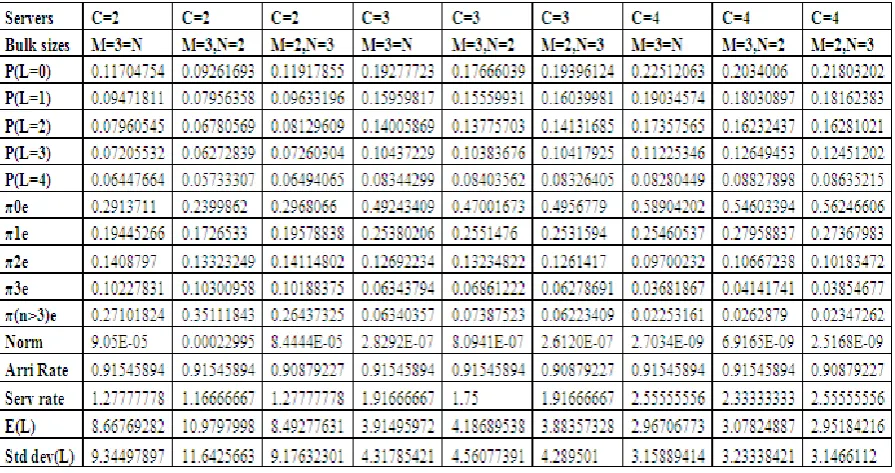
The bulk size service probabilities are given in table 1for the case when M = N = 3 for the two environment. For the case M =3, N=2 the probabilities of bulk service size 2 in E1 is fixed as .5 and of bulk size 3 in E1 is fixed as 0; and other probabilities are unchanged.
Table 1: Service probabilities
Environment 1 P(size 1) P(size 2) P(size 3) Environment 2 P(size 1) P(size 2) P(size 3)
Service .5 .3 .2 Service .8 .2 0
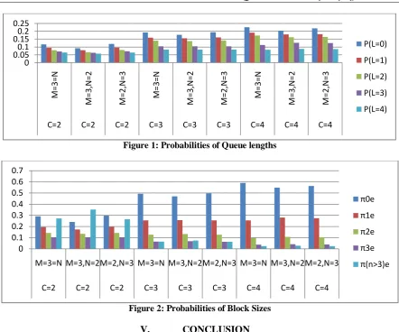
Thirty iterations are performed for all the models to iterate the rate Matrix R and the norms of convergence are recorded. Queue length probabilities and block size probabilities are calculated. Expected queue length and Standard deviation are presented. They show significant variations when M, N and C are changed. The probabilities of queue lengths and block sizes are presented in figures 1 and 2 for all the nine examples.
Figure 1: Probabilities of Queue lengths
Figure 2: Probabilities of Block Sizes
V. CONCLUSION
Two BMAP/M/C bulk service queues and their sub cases with randomly varying environments have been studied. The environment changes the batch Markovian arrival processes, the service rates, and the probabilities of bulk services. Matrix geometric ( modified matrix geometric) results have been obtained by suitably partitioning the infinitesimal generator by grouping of customers, environments, BMAP and PH phases together respectively when the number of servers is not greater than ( greater than) the maximum of the maximum arrival and maximum service sizes. The basic system generators of the queues are block circulant matrices which are explicitly presenting the stability condition in standard form. Numerical results for various bulk queue models are presented and discussed. Effects of variation of rates on expected queue length and on probabilities of queue lengths are exhibited. The decrease in arrival rates (so also increase in service rates) makes the convergence of R matrix faster which can be seen in the decrease of norm values. Bulk BMAP/PH/C queue with randomly varying environments causing changes in sizes of the PH phases may produce further results if studied since BMAP/PH/C queue is a most general form almost equivalent to G/G/C queue.
VI. ACKNOWLEDGEMENT
The fourth author thanks ANSYS Inc., USA, for providing facilities. The contents of the article published are the responsibilities of the authors.
REFERENCES
[1]. Rama Ganesan, Ramshankar.R and Ramanarayanan. R (2014) M/M/1 Bulk Arrival and Bulk Service Queue with Randomly Varying Environment, IOSR-JM, Vol.10,Issue 6, Ver III, Nov-Dec, 58-66 [2]. Sandhya.R, Sundar.V, Rama.G, Ramshankar.R and Ramanarayanan.R, (2015) M/M//C Bulk Arrival And
Bulk Service Queue With Randomly Varying Environment,IOSR-JEN,Vol.05,Issue02,||V1||,pp.13-26. [3]. Ramshankar.R, Rama Ganesan and Ramanarayanan.R (2015) PH/PH/1 Bulk Arrival and Bulk Service
Queue ,IJCA, Vol. 109,.3,27-33
[4]. Ramshankar.r, Rama.G, Sandhya.R, Sundar.V, Ramanarayanan.R , (2015), PH/PH/1 Bulk Arrival and Bulk Service Queue with Randomly Varying Environment, IOSRJEN, Vol.05,Issue.02,||V4|| pp.01-12. [5]. Bini.D, Latouche.G and Meini.B (2005). Numerical methods for structured Markov chains, Oxford Univ.
Press, Oxford. 0
0.050.1 0.150.2 0.25
M=3
=N
M=
3,
N
=2
M=
2,
N
=3
M=
3=N
M=3
,N
=2
M=
2,
N
=3
M=
3=N
M=
3,
N
=2
M=
2,
N
=3
C=2 C=2 C=2 C=3 C=3 C=3 C=4 C=4 C=4
P(L=0)
P(L=1)
P(L=2)
P(L=3)
P(L=4)
0 0.1 0.2 0.3 0.4 0.5 0.6 0.7
M=3=N M=3,N=2M=2,N=3 M=3=N M=3,N=2M=2,N=3 M=3=N M=3,N=2M=2,N=3
C=2 C=2 C=2 C=3 C=3 C=3 C=4 C=4 C=4
π0e
π1e
π2e
π3e
[6]. Chakravarthy.S.R and Neuts. M.F.(2014). Analysis of multi-server queue model with MAP arrivals of customers, SMPT, Vol 43,79-95,
[7]. Gaver, D., Jacobs, P., Latouche, G, (1984). Finite birth-and-death models in randomly changing environments. AAP. 16, 715–731
[8]. Latouche.G, and Ramaswami.V, (1998). Introduction to Matrix Analytic Methods in Stochastic Modeling, SIAM. Philadelphia.
[9]. Neuts.M.F.(1981).Matrix-Geometric Solutions in Stochastic Models: An algorithmic Approach, The Johns Hopkins Press, Baltimore
[10]. Lucantony.D.M. (1993), The BMAP/G/1 Queue: A tutorial, Models and Techniques for Performance Evaluation of Computer and Communication Systems, L. Donatiello and R. Nelson Editors, Springer Verlag, pp 330-358.
[11]. Cordeiro.J.D and Kharoufch. J.P, (2011) Batch Markovian Arrival Processes,
www.dtic.mil/get-tr-doc/pdf?AD=ADA536697 & origin=publication Detail.
[12]. Usha.K,(1981), Contribution to The Study of Stochastic Models in Reliability and Queues, PhD Thesis, Annamlai University,India.
[13]. Usha.K,(1984), The PH/M/C Queue with Varying Environment, Zastosowania Matematyki Applications Mathematicae, XVIII,2 pp.169-175.