Scalable
SOCP-based
localization
technique
for
wireless
sensor
network
Randa M. Abdelmoneem
1, Eman Shaaban
1,*1DepartmentofComputerSystems,FacultyofComputerandInformationSciences,Ain-ShamsUniversity,Egypt
Abstract
Node localization is one of the essential requirements to most applications of wireless sensor networks. This paper presents a detailed implementation of a centralized localization technique for WSNs based on Second Order Cone Programming (SOCP). To allow scalability, it also proposes a clustered localization approach for WSNs based on that centralized SOCP technique. The cluster solves the SOCP problem as a global minimization problem to get positions of the cluster sensor nodes. To enhance localization accuracy, a cluster level refinement step is implemented using Newton optimization. The initial position for the Gauss-Newton optimization is the position drawn from the preprocessor SOCP localization. The proposed approach scales well for large networks and provides a considerable reduction in computation time while yielding good localization accuracy.
Receivedon 21 September 2015;acceptedon 04 November 2015;publishedon 01 January 2016 Keywords: wireless sensor network, localization, second-order cone programming
Copyright © 2016 E. Shaaban and R. M. Abdelmoneem, licensed to EAI. This is an open access article distributed under the terms of the Creative Commons Attribution license (http://creativecommons.org/licenses/by/3.0/), which permits unlimited use, distribution and reproduction in any medium so long as the original work is properly cited. doi:10.4108/eai.1-1-2016.150815
1. Introduction
A wireless sensor network (WSN) is a group of a few to several hundreds or even thousands of sensor nodes deployed over a significant area. WSNs have a wide range of applications which include environmental monitoring, target tracking, home automation, military applications and others. To process sensor data in WSN, it is imperative to know where the data is coming from. So, knowledge of nodes locations is an essen-tial requirement for many location-aware applications including aforementioned applications, location-based services (LBS) and location-based routing. Several sur-veys discussed localization strategies and attempted to classify different localization techniques like [1],[2],[3]. Localization techniques could be classified according to all calculations being performed on a single node or distributed on all the network sensor nodes to cen-tralized localization technique (e.g. MDS-MAP [4] and Semi-Definite programming (SDP) [5]) and distributed localization technique (e.g. APIT [6]). Another new
∗
Corresponding author. Email:[email protected]
approach in this classification is called locally cen-tralized or cluster-based localization techniques which are distributed techniques that achieve a global goal by communicating with nodes in some neighbourhood only. According to the process of estimating node-to-node distances or angles, the localization techniques are classified to range-based and range-free localization techniques. Range-based localization techniques are based on distances measurements between the nodes using Time of Arrival (TOA), time difference of arrival (TDOA) and received signal strength (RSS) (e.g. Tri-lateration) or based on angles between the nodes like angle of arrival (AOA) (e.g. Triangulation) [7]. Range-free localization techniques depend on network con-nectivity (e.g. DV-HOP) [6] to indirectly obtain the distances between the nodes. Also, localization tech-niques can be classified to based or anchor-free localization techniques. Anchor-based localization techniques usually provide absolute positions for the nodes whereas anchor-free localization techniques pro-vide relative positions. Biswas and Ye who proposed a semi-definite programming (SDP) relaxation of the localization problem which has various nice proper-ties [5]. SOCP-based localization technique was studied
1
on Industrial Networks and Intelligent Systems
Research Article
and Intelligent Systems 09 2015 -01 2016 | Volume 3 | Issue 6 | e5
EAI Endorsed Transactions on Industrial Networks
by Tseng [8] who provided a second order cone pro-gramming (SOCP) relaxation of localization problem, motivated by its simpler structure and its potential to be solved faster than SDP. This paper proposes a locally centralized technique for solving the sensor network localization problem. It is a Refined Clustered technique based on Second-Order Cone Programming (RC-SOCP). The proposed approach divides the large network into smaller sub networks. For each cluster, the cluster solves the SOCP problem as a global minimiza-tion problem to get initial posiminimiza-tions of the cluster sensor nodes. To enhance localization accuracy, a cluster level refinement step is implemented using Gauss-Newton optimization. The initial position for the GaussNewton optimization is the position drawn from the preproces-sor SOCP localization. Rest of the paper is organized as follows: Section 2 introduces the centralized SOCP localization technique. Proposed technique is presented in section 3. Simulation results and evaluations are presented in section4and we conclude in section5.
2. Centralized SOCP localization technique
This section discuses a detailed description of SOCP problem formulation for Castalia wireless sensor net-works simulator, providing the formulation algorithm and solver tools. It also investigates the results obtained.
2.1. Problem formulation
Second-order cone programming relaxation method for wireless sensor network localization was first studied by Tseng [8]. In this methodn is the total number of nodes inRd (d ≥1), m are the nodes whose locations xi ∈R2, i =1,...,m are to be determined givenn-mnodes called anchors with known locations and dij which is the euclidean distance between nodes i and j where (i,j) ∈ A. A is the undirected neighbour set defined
asA:={(i, j) :||xi−xj|| ≤RadioRange}. The problem is
formulated as the non-convex minimization equation
υopt =min
X
(i,j)∈A
|yij−d2
ij| (1)
s.t. yij =||xi −xj||2 ∀(i, j)∈ A
Where || . || denotes the euclidean norm. Then
in order to yield a convex-problem, the equality constraints are relaxed to non-equality constraints, the problem becomes
υopt =min
X
(i,j)∈A
|yij−d2
ij| (2)
s.t. y ≥ ||x −x||2 ∀(i, j)∈ A
Equation (2) can be rewritten as
min X i,j∈A
Uij (3)
s.t. yij ≥ ||xi−xj||2 ∀(i, j)∈ A
uij≥ |yij−dij2| ∀(i, j)∈ A
uij ≥0
2.2. Centralized SOCP localization implementation
Given a wireless sensor network with size n sensors, m are sensors with unknown locations, n−m are
sensors with known locations (anchors). To solve this localization problem, the centralized SOCP localization technique is performed in three phases. In the first phase, nodes estimate their distances with sensor and anchor neighbours which are within their communication ranges. The second phase involves wireless communication and routing between the nodes. In the third phase, the positions matrix and the lower triangle of the distances matrix are created with sizes 2×n, n×n respectively and filled with their
relevant data received from the nodes. Distances Matrix
0 0 0 .. 0
d10 0 0 .. 0 d20 d21 0 .. 0 .. .. .. .. 0 dn0 dn1 .. .. 0
wheredijis the euclidean distance between nodesi,j.
Positions Matrix
x0 x1 x2 .. xn y0 y1 y2 .. yn
!
wherexi,yiare the x,y co-ordinates of an anchor node or 0,0 if the sensor node is not an anchor. Algorithm
1 shows the pseudo-code of formulating the SOCP-localization problem according to equation (3). For a network of n total nodes and m non-positioned nodes, there are Ω(m) variables and Ω(m) inequality constraints using position and distance matrices [8].
2.3. Simulator and Solver Tools
Algorithm 1 : formulating the SOCP-localization problem
1: procedure CREATEMODEL(distanceMatrix, positions-Matrix)
2: Let model = model of the problem , vars = array of variables
3: for alldij indistanceMatrixdo
4: #Read positions of nodes i,j from positions matrix
5: x1pos←positionsMatrix[0][i] 6: y1pos←positionsMatrix[1][i] 7: x2pos←positionsMatrix[0][j] 8: y2pos←positionsMatrix[1][j]
9: ifx1pos! = 0 ory1pos! = 0then #Check node i being anchor
10: node i isAnchor 11: else
12: # Search for variables in vars array and if not found create, add them
13: ifvariables ofiinvars then
14: xi ←vars[i].x,yi ←vars[i].y
15: else
16: create varsxi, yi
17: vars.add(xi) ,vars.add(yi) 18: end if
19: end if
20: Repeat steps 7-17 for the second node j
21: # If at least one of the nodes is not an anchor complete model formulation
22: if node i isAnchor==false Or node j isAnchor==false then
23: create variablesuij, yij 24: vars.add(uij) ,vars.add(yij)
25: objectiveExpression←objectiveExpression+uij 26: create constraint c
27: c.expression←yij−uij 28: c.lowerbound←0 29: c.upperbound ←dij∗dij 30: model.add(c)
31: end if
32: # Create quadratic constraint. Substitue with position values for anchor node(s) if found
33: if node i isAnchor==false And node j isAnchor==false then
34: expr ←y−(xi−xj)∗(xi−xj)−(yi −yj)∗
(yi−yj)
35: else if node i isAnchor==true And node j isAnchor==false then
36: expr ←y−(x1pos−xj)∗(x1pos−xj)−
(y1pos−yj)∗(y1pos−xj)
37: else if node i isAnchor==false And node j isAnchor==true then
38: expr ←y−(xi−x2pos)∗(xi −x2pos)−(yi− y2pos)∗(yi −y2pos)
39: end if
Algorithm 1Continue 40: create constraint q 41: q.expression←expr 42: q.lowerbound←0 43: q.upperbound← ∞ 44: model.add(q) 45: end for
46: create objective obj 47: obj.f n←minimization
48: obj.expression←objExpression 49: model.add(obj)
of low power embedded devices such as wireless sensor nodes [13]. Our simulation study is carried out using version 3.2 of Castalia which build upon version 4.1 of OMNet++.
The implementation of our SOCP-based localization technique uses IBM ILOG CPLEX. IBM LOG Concert Technology (modelling layer) C++ Interface Of OPL was used to integrate our problem model in Castalia with the CPLEX solver[15].
2.4. Performance Evaluation
We evaluate the performance of the centralized SOCP-based localization by measuring localization accuracy, computation time and problem size.
The mean error between the estimated and the true location of the non-anchor nodes in the network is adopted as the performance metric. It is defined as follows
LE= 1 N.
N
X
i=1
kˆxi−xik
Where LE denotes a localization error, N denotes the number of nodes in a network whose location is estimated, xi is the true position of the node i in the network , ˆxiis estimated location of the node i (solution of the location system).
Computation time is defined as the time spent for formulating and solving the SOCP problem at the sink node and it is measured using C++ std.clock() function. The time needed for computing the relative distances at the nodes and communication or message exchanges time is excluded. Problem size corresponds to number of variables and constraints for the SOCP-localization problem formulated at the sink node.
We evaluate performance of the centralized SOCP-based localization technique by studying the effect of varying Network size (number of nodes), Anchors percentage, Communication radio range and Noise value added to distances measurements.
Anchors
Anchors are chosen to form a convex hull distribution around the sensor nodes in the network. This
3 and Intelligent Systems
09 2015 -01 2016 | Volume EAI Endorsed Transactions on Industrial Networks
distribution was chosen to assure good localization accuracy when non-anchor nodes are in the convex hull of the anchors [11].
Radio range
Radio range is specified by replacing the path loss parameterP L(d) of the log-normal shadowing model in equation (4)
P L(d) =P L(d0) + 10.η.log( d d0
) +Xσ (4)
with its equivalent
P L(d) =PT x−PRx
Equation(4) calculates the average path loss in the chan-nel model in Castalia [13]. Setting the random variable Xσ to 0 for the case of no fading, thus simulating general environment conditions where stationary WSN is deployed in fairly static environments and fading is not very significant, thus it is ignored. η is sub-stituted with 2.4 which is typical default value that will produce results similar to many outdoors (and sometimes indoors) environments.d is the path length allowing communications between two paired nodes, thus representing the radio range. So, the radio range can be specified by
RR= 10PT x−PRx−P L(d0)/24 (5)
PRx is inferred from ReceiverSensetivity value of the radio card chosen (radio model for CC2420 chip by Texas instrument) and is qual to -95 dBm. So the radio range is mainly controlled by the transmit power and the path loss at reference distance values specified according to
RR= 10PT x+95−P L(d0)/24 (6)
The degree of connectivity is controlled by the radio range specified. It is calculated as the average connectivity of all the nodes which is equivalent to the average number of neighbours for all of the sensor nodes in the network for a specific radio range and environment area.
Noise to distance
We added normally distributed measurement noise to the true distance according to the equation
dij=||xi−xj||.max{ 0,1 +ij.nfd } ∀(i, j)∈ A
Where ij is a normal random variable N(0, 1) representing measurement noise andnf d∈[0, 1] is the
noise factor (standard deviation of the distance error in percentage) for the distance measurements [9].
2.5. Simulation Results
Simulations are conducted for a randomly generated 500 nodes uniformly distributed on the unit square area
[-0.5, 0.5]2 with noise factor (nf d)=0.05, radio range (rr)=0.17 and Degree of Connectivity=38. Anchors are chosen to form a convex hull distribution around the sensor nodes in the network with percentage (p) of 15%. Simulations are averaged over 10 runs with confidence level of 95%. Simulations were carried out on a PC with 2.4 GHz Quad-Core processor and 4 GB RAM using Castalia simulator integrated with IBM CPLEX solver using C++ interface.
Fig.?? shows a snapshot of the true sensor positions and the estimated positions. True positions of the sensors are depicted in blue coloured points and the estimated node positions are depicted in red coloured points, solid lines indicate the error between the estimated and true sensor positions. A close match is observed between the estimated and true positions. The estimated positions become less accurate as we move towards the boundary. Fig.1b shows the Commulative distributive function (CDF) of localization errors. The
(a)Snapshot of the true vs estimated nodes locations
(b)CDF of localization errors
Figure 1. Centralized SOCP results for uniform topology: n = 500,RadioRange=0.17, p =0.15 andnf d =0.05.
Fig.1is 0.02 with confidence interval (-0.002 , 0.04) and standard deviation 0.04 .
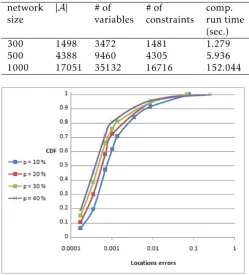
Effect of Varying Network Size. Fig.2 shows the CDF of localization errors (log scale) for different network sizes with the same radio range in the same area for a network withnf d=0.05,rr=0.11 and anchor percentage of 15%. Fig.2 shows that when the network size increases in the same area, the degree of connectivity is increased and this leads to larger communications between nodes. Consequently, more distances are obtained between nodes which directly improves the localization accuracy. On the other hand, it must be noted that increasing node density and hence communications between nodes increases network overhead and energy consumption.
The mean localization errors (LEs), and their
Figure 2. CDF of localization errors (log scale) for different network sizes
confidence intervals are listed in table1which shows a decrease in mean localization error when increasing the network size. Table 2 shows the number of variables, number of constraints, and the computation runtime spent for solving the networks in Fig.2. Computation runtime grows with increasing network size, thus limits the scalability of the technique for large networks.
Table 1. Mean localization errors for different network sizes
network mean standard confidence
size error deviation interval
300 0.01 0.022 ( -0.001 , 0.025)
500 0.006 0.015 ( -0.003 , 0.016)
1000 0.002 0.018 ( -0.009 , 0.014)
Effect of Varying Anchors Percentage. Fig.3 shows the effect of changing anchor percentage on the localization accuracy for a network of 500 nodes, rr=0.17 and nf d=0.05. We changed number of anchor nodes while maintaining number of non-positioned nodes the
Table 2. Performance and computation runtime comparison of different network sizes.
network |A| # of # of comp.
size variables constraints run time
(sec.)
300 1498 3472 1481 1.279
500 4388 9460 4305 5.936
1000 17051 35132 16716 152.044
Figure 3. CDF of localization errors (log scale) for different percentage of anchors
same (500 non-positioned nodes). Fig.3 shows that increasing anchor percentage considerably increases the localization accuracy. For a network of 20% of anchors, 80% of the nodes have error less than 0.0017. For anchor percentage greater than 20%, slight improvement in localization accuracy is achieved. This means that the implemented technique requires a proper setting of percentage of anchors to achieve good localization accuracy. The mean localization errors (LEs) and their confidence intervals are listed in table3. However, increasing anchors percentage increases the
Table 3. Mean localization errors for different anchor percentages
anchor mean standard confidence
percentage error deviation interval
10% 0.003 0.006 (-0.001 , 0.006)
20% 0.002 0.005 (-0.001 , 0.005)
30% 0.0018 0.0045 (-0.001 , 0.0048)
40% 0.0015 0.0046 (-0.001 , 0.0044)
total complexity of the computations. This is shown in table4.
Effect of Varying Communication Radio Range. To study the effect of changing radio range on localization
5 and Intelligent Systems
09 2015 -01 2016 | Volume EAI Endorsed Transactions on Industrial Networks
Table 4. Performance and computation runtime comparison of different anchor percentages.
anchor |A| # of # of comp.
percentage variables constr- run time
aints (sec.)
10% 12590 25970 12485 35.32
20% 15013 30370 14685 66.39
30% 17611 34566 16783 94.56
40% 20198 38306 18653 124.71
accuracy, we set rr to 0.08, 0.1 and 0.15. Fig.4
Figure 4. CDF of localization errors (log scale) for different radio ranges
shows that networks with lower radio range have higher localization error. This is due to less inter-node communications and hence distances information between nodes. It must be noted that for rr=0.08, 97% of total nodes are localized (413 node) whereas 100% of total nodes are localized for rr=0.1, 0.15. However, increasing radio range increases power consumption and adds more communication overhead to the network. The mean localization errors (LEs) and their confidence intervals are listed in table 5. Performance and computation runtime comparison is shown in table6.
Table 5. Mean localization errors and computation time for different radio ranges
radio mean standard confidence
range error deviation interval
0.08 4.2 16.7 ( -6.15 , 14.5)
0.1 0.015 0.034 ( -0.006 , 0.036)
0.15 0.004 0.009 ( -0.002 , 0.01)
Effect of Varying Noise Value Added to Distances Measurements. Fig.5 shows the effect of changing nf d on the localization accuracy. Fig.5shows that there is no
Table 6. Performance and computation runtime comparison of different radio ranges.
radio |A| # of # of comp.
range variables constraints run time
(sec.)
0.08 982 2750 965 0.62
0.1 3668 8052 3601 4.58
0.15 7819 16172 7661 29.82
Figure 5. CDF of localization errors (log scale) for differentnf d
significant improvement in localization accuracy when decreasing nf d. Thus, the implemented localization technique solves the localization problem with good localization accuracy in the presence of inaccuracies in distance measurements. The mean localization errors (LEs) and their confidence intervals for the networks in Fig.5are listed in table7.
Table 7. Mean localization errors for differentnf d
nf d mean standard confidence
error deviation interval
0.05 0.003 0.007 ( -0.001 , 0.007)
0.1 0.005 0.009 ( -0.0008 , 0.01)
0.15 0.006 0.01 ( -0.0005 , 0.012)
0.2 0.007 0.012 (-0.0001 , 0.014)
3. RC-SOCP: Proposed refined clustered SOCP
localization approach
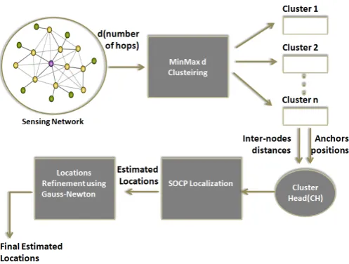
performance by reducing computation time, energy consumption, and communication overhead resulting from numerous communications overhead between the nodes in centralized localization approach. Its architecture is divided into three phases as shown in Fig.6: clustering phase, localization phase and refinement phase. In the first phase, Min-Max d clustering algorithm is used to divide the network and select the CH according to the IDs of the nodes. In the second phase, each cluster implements SOCP-based localization technique to localize the member nodes including the CH itself. In the third phase, each cluster implements Gauss Newton local algorithm to refine the estimated locations obtained.
Figure 6. Refined Clustered SOCP Architecture
3.1. Clustering
Min-Max d clustering algorithm is used to divide the network and select the cluster head CH according to the IDs of the nodes. It was chosen because it is a simple, less computationally demanding and thus doesn’t add extra complexity to the localization technique. This clustering algorithm runs asynchronously eliminating overhead of synchronizing the clocks of the nodes. Also, a low variance in cluster sizes leads to better load balancing among the cluster-heads [10].
3.2. Implementing SOCP on cluster-head
At the end of the clustering phase, the network is divided into multiple independent clusters. Each cluster of sizeCN sensors,CM sensors with unknown locations and CN−CM sensors with known locations
(anchors). Member nodes send their relevant distance information with their neighbours to their elected
CHs. Each CH constructs the positions matrix and the lower triangle of the distance matrix of sizes 2×CN,
CN×CN respectively as in centralized technique then
formulates SOCP localization problem for its cluster member nodes according to algorithm 1 and uses CPLEX optimization solver to estimate the positions of the nodes.
3.3. Refinement phase
To enhance localization accuracy of clustered SOCP (C-SOCP), a cluster level refinement step is implemented. Each cluster head solves the network localization problem using Gauss-Newton (iterative least-squares) algorithm [11]. The initial position guess for the Gauss-Newton optimization is the positions drawn from the preprocessor SOCP solver which is close to the global solution. Given m residual functions r= (r1, ..., rm) of n variables X= (X1, ..., Xn), with m≥n, a non-linear least square problem is an unconstrained optimization problem of the form
min m
X
i=1
ri(X)2. (7)
The Gauss-Newton algorithm iteratively finds the minimum of the sum of the squares in equation(7). For implementing the Gauss-Newton method as a refinement step, where X refers to the position coordinates of the sensor node (x,y), and hence n is set to 2. m is the number of residuals, and is equal to the number of anchor neighbours to that sensor node. The residual functionri is defined as
ri =||X−a||2−d2 (8)
Where a represents the positions of the anchor node (ax, ay) and d is the estimated distance between the sensor node and the non-positioned node. Starting with an initial guess X(0) for the minimum, the method proceeds by the iterations
X(s+1)=X(s)−JrTJr−1JrTr(X(s)) (9)
Where the symbolTdenotes the matrix transpose. If r
and X are column vectors, the entries of the Jacobian matrix are
(Jr)ij =
∂ri(X(s)) ∂Xj
(10)
The derivative of the residual function to the first variablexis:
∂ri(X(s))
∂x =
(x−x0) ri(X(s))
And the derivative of the residual function to the second variableyis:
∂ri(X(s))
∂y =
(y−y0) ri(X(s))
7 and Intelligent Systems
09 2015 -01 2016 | Volume EAI Endorsed Transactions on Industrial Networks
Algorithm 2: Gauss-Newton Algorithm
1: procedure GAUSSNEWTON(distanceMatrix, positions-Matrix)
2: Let iters = number of iterations , neighbours = array of anchor neighbours
3: for allnodei do
4: ix←initial guess of x coordinate for node i 5: iy ←initial guess of y coordinate for node i 6: n←number of neighbours of node i 7: neighbours←getNeighboursOfNode(i)
8: Let distanceEstimate = array of distances estimations with anchor neighbours of sizen×1 9: Let distanceNoise = array of distances noises
between estimated distances and distances of initial guessn×1
10: Let J = jaccobian matrix of sizen×2
11: LetJT = transpose Jacobian matrix of size 2×n 12: Let delta = matrix of size 2×1 of values for
updating x,y coordinates of node i 13: forj= 0 toitersdo
14: fork= 0 tondo
15: xdif f ←ix−neighbours[k].x 16: ydif f ←iy−neighbours[k].y 17: distance←pow(xdif f ,2) +
pow(ydif f ,2)
18: distanceEstimate(k,0)←sqrt(distance) 19: J(k,0)←xdif f /distanceEstimate(k,0) 20: J(k,1)←ydif f /distanceEstimate(k,0) 21: distance←distanceMatrix[i, k]
22: distanceEstimate(k,0)←distanceNoise(k,0)
- distance 23: end for
24: delta←( ( ( (JTJ)JT ).inverse() )JT )distanceN oise 25: ix←ix−delta(0,0)
26: iy←iy−delta(1,0) 27: end for
28: end for
Algorithm 2 shows the pseudo-code of the Gauss-Newton algorithm for refining the locations obtained from C-SOCP.
3.4. Performance evaluation of RC-SOCP
RC-SOCP performance is evaluated by measuring localization accuracy and computation time. The localization accuracy is calculated as defined in section 2.4. To calculate RC-SOCP computation time, we calculate C-SOCP runtime and Gauss-Newton refinement algorithm runtime on each CH. The computation time metric is measured as the maximum RC-SOCP computation time among CHs. C-SOCP runtime is the time spent for formulating and solving the SOCP problem on the CH using C++ std.clock() function. The time needed for computing the relative distances at the nodes and communication or message exchanges time is excluded. We evaluate
the performance of RC-SOCP localization technique by studying the effect of varying: cluster size , anchor percentage, communication radio range, noise value added to distances measurements.
4. Simulation results
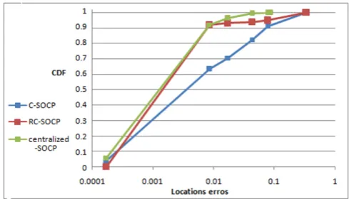
Simulations are conducted for a randomly generated 500 nodes uniformly distributed on the unit square area [-0.5, 0.5]2 with noise factor(nf d) = 0.05, radio range(rr) = 0.17, d = 3 and Degree of Connectivity = 37. Anchors are chosen to be uniformly distributed throughout the network with percentage(p) of 30%. Number of Gauss-Newton iterations is 25. Simulations are averaged over 10 runs with confidence level of 95%. Figs. (7a) and (7b) show a snapshot of the true sensor positions and the estimated positions of the C-SOCP and RC-SOCP respectively. True positions of the sensors are depicted in blue colored points and the estimated node positions are depicted in red colored points, solid lines indicate the error between the estimated and true sensor positions. An improvement in localization accuracy is observed for RC-SOCP compared to C-SOCP. It is also observed that the estimated positions become less accurate as we move towards the boundaries of the clusters in C-SOCP which is greatly refined in RC-SOCP. The mean localization error (LE) for the network in fig.
7 using C-SOCP is 0.02 and standard deviation 0.04, and LE is 0.01 and standard deviation 0.04 for RC-SOCP. This clarifies that the mean error is reduced by 50% using RC-SOCP. Fig.7c shows a comparison between the Commulative distributive function (CDF) of localization errors resulting from centralized-SOCP localization implemented in section2, C-SOCP and RC-SOCP. The detailed CDF of localization errors for the results in fig.7care listed in table8.
(a) Snapshot of real vs estimated nodes locations of C-SOCP localization
(b) Snapshot of real vs estimated nodes locations of RC-SOCP localization
(c)CDF results of localization errors(log scale) of centralized SOCP, C-SOCP and RC-SOCP sizes
Figure 7. C-SOCP and RC-SOCP results for uniform topology:
n= 500, rr = 0.17, p= 0.15, d= 3andnf d = 0.05.
Table 8. CDF results of localization errors
Locali- technique nodes mean stand.
zation perce- error dev.
error tage
<0.004
C-SOCP 55.5% 0.001 0.001
RC-SOCP 70% 0.002 0.0009
centralized-SOCP 87% 1.07e-1 0.0001
<0.006
C-SOCP 59.9% 0.001 0.0016
RC-SOCP 90% 0.0029 0.0013
centralized-SOCP 90% 0.001 0.121
<0.07
C-SOCP 91% 0.01 0.016
RC-SOCP 95% 0.0039 0.005
centralized-SOCP 99.5% 0.0025 0.118
<0.2
C-SOCP 98% 0.019 0.03
RC-SOCP 98% 0.0077 0.02
centralized-SOCP 100% 0.0026 0.118
<0.35 C-SOCP 100% 0.02 0.038
RC-SOCP 100% 0.01 0.04
centralized-SOCP 100% 0.0026 0.118
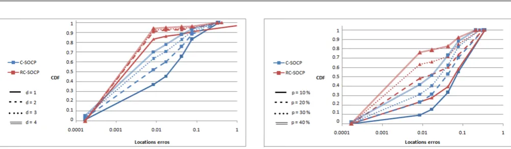
4.1. The effect of varying cluster Size
To study the effect of varying cluster size on localization error and computation time, we set the number of consecutive hops (d) to 1, 2, 3 and 4. Fig.8 shows CDF of localization errors (log scale) for C-SOCP and RC-SOCP with different d. Table 9 shows number of clusters, C-SOCP runtime, Gauss-Newton run-time and RC-SOCP runrun-time of networks. Fig.8 shows that the refinement phase of RC-SOCP enhances the result of the preprocessor C-SOCP. C-SOCP is highly dependent on cluster size compared to RC-SOCP. As the cluster size increases, the localization accuracy is improved since more nodes distances information is obtained at the CH. These distances information directly affect and enhance the formulation of the sub problems and hence improve the result of the SOCP problem solver. However, increasing cluster size increases the problem size and computation time and communication overhead of the cluster. For RC-SOCP, the localization accuracy is increased when d is increased from 1 to 2. For d≥2, there is
not significant difference in localization accuracy for different cluster size (d), since refinement algorithm reaches the optimal solution for the estimate of locations of the nodes. So, adjusting cluster size using d= 2 which is approximated to number of clusters around 11 in this network size(500 nodes) as shown in table 9 yields good accepted localization accuracy. Table 9 shows that incrementing the cluster size d reduces the number of clusters approximately to the
9 and Intelligent Systems
09 2015 -01 2016 | Volume EAI Endorsed Transactions on Industrial Networks
Figure 8. CDF reaults of localization errors (log scale) for different cluster sizes
half. As a result of increasing cluster sizes, C-SOCP and RC-SOCP run times are increased while Gauss-Newton runtime has no significant change. Table 10
Table 9. Performance and computation runtime comparison of different cluster sizes.
d # of C-SOCP Gauss-Newton RC-SOCP
clusters runtime runtime runtime
(sec.) (sec.)
1 24 2.117 0.014 2.128
2 11 6.468 0.011 6.475
3 7 14.761 0.019 14.791
4 5 20.554 0.016 20.57
Table 10. Mean localization errors for different cluster sizes for C-SOCP and RC-SOCP
d technique mean standard confidence
error deviation interval
1 C-SOCP 0.03 0.04 ( 0.009 , 0.06 )
RC-SOCP 0.02 0.13 (-0.05 , 0.11 )
2 C-SOCP 0.028 0.04 ( 0.002 , 0.05 )
RC-SOCP 0.015 0.05 ( -0.016 , 0.047 )
3 C-SOCP 0.02 0.038 ( -0.002 , 0.045 )
RC-SOCP 0.013 0.04 ( -0.01 , 0.04 )
4 C-SOCP 0.016 0.033 ( -0.004 , 0.037)
RC-SOCP 0.01 0.036 ( -0.01 , 0.03)
also shows that increasing the cluster size reducesLE in C-SOCP significantly for all d whereas it leads to slightly improvedLEin RC-SOCP ford≥2.
4.2. The effect of varying anchors percentage
To investigate the effect of varying anchors percentage on localization error and computation time, we change number of anchor nodes to 10%, 20%, 30% and
Figure 9. CDF results of localization errors(log scale) for different anchors percentage
40% of the number of non-positioned nodes while maintaining the number of non-positioned nodes the same (500 non-positioned nodes), rr = 0.11 , d = 2 and nf d = 0.05 for C-SOCP and RC-SOCP. Fig.9
shows that increasing anchors percentage considerably increases the localization accuracy for both C-SOCP and RC-SOCP; and RC-SOCP has good localization accuracy compared to C-SOCP. Appropriate percentage of anchors ensures that each cluster has an acceptable number of anchors to perform the localization problem. However, increasing number of anchors often imposes additional costs. Table 11 shows that the number of clusters and computation runtime time are increased with increasing the number of anchors. This happens due to the increase of the total number of nodes in the network. Table 12 shows a reduction in LE when increasing anchors percentages in both C-SOCP and RC-SOCP.
Table 11. Performance and computation runtime comparison of different anchors percentages.
anchor # of C-SOCP Gauss-New RC-SOCP
percen- clust- runtime ton runtime runtime
tage ers (sec.) (sec.) (sec.)
10% 20 0.356 0.011 0.365
20% 24 0.393 0.016 0.405
30% 26 0.465 0.012 0.476
40% 27 1.693 0.022 1.71
4.3. The effect of varying communication radio range
To study the effect of changing radio range on localiza-tion accuracy, we setrrto 0.08, 0.1, 0.15 and 0.17. Fig.10Table 12. Mean localization errors for different anchors percentages for C-SOCP and RC-SOCP
anchor technique mean standard confidence
percentage error deviation interval
10% C-SOCP 0.08 0.06 ( 0.042 , 0.118 )
RC-SOCP 0.083 0.07 ( 0.035 , 0.1 )
20% C-SOCP 0.05 0.048 ( 0.02 , 0.08 )
RC-SOCP 0.052 0.137 ( -0.03 , 0.137 )
30% C-SOCP 0.03 0.04 ( 0.01 , 0.06 )
RC-SOCP 0.038 0.1 ( -0.036 , 0.1 )
40% C-SOCP 0.02 0.03 ( 0.007 , 0.04 )
RC-SOCP 0.02 0.07 ( -0.02 , 0.06 )
Figure 10. CDF results of localization errors (log scale) for different radio ranges
for Gauss-Newton iterations. Large radio ranges lead to higher localization accuracy. However, increasing radio range increases power consumption, and adds more communication overhead. Average degree of connectiv-ity (doc), number of clusters and run-times of networks in fig.10are shown in table13.
Table 13. Performance and computation runtime comparison of different radio ranges.
radio doc # of SOCP Gauss- RC-SOCP
range clust- runtime Newton runtime
ers (sec.) run time (sec.)
(sec.)
0.08 3 63 0.148 0.013 0.162
0.1 12 48 0.595 0.013 0.601
0.15 28 14 1.592 0.013 1.605
0.17 37 11 6.468 0.011 6.475
4.4. The effect of varying noise value added to
distances measurements
Fig.11shows that RC-SOCP is highly affected bynf d compared to C-SOCP while RC-SOCP has a good localization accuracy compared to C-SOCP for allnf ds.
Table 14. Mean localization errors for different radio ranges for C-SOCP and RC-SOCP
radio technique mean stand- confidence
range error ard dev- interval
iation
0.08 C-SOCP 0.032 0.02 ( 0.02 , 0.05)
RC-SOCP 0.038 0.08 ( -0.01 , 0.09)
0.1 C-SOCP 0.032 0.04 ( 0.017 , 0.07)
RC-SOCP 0.025 0.13 ( -0.04 , 0.12)
0.15 C-SOCP 0.032 0.04 ( 0.005 , 0.06 )
RC-SOCP 0.02 0.05 ( -0.01 , 0.05 )
0.17 C-SOCP 0.028 0.04 ( 0.002 , 0.05 )
RC-SOCP 0.015 0.05 ( -0.02 , 0.05 )
A slight improvement in localization accuracy for C-SOCP is noticed when decreasingnf dwhile significant improvement in localization accuracy is noticed when decreasingnf din RC-SOCP. The localization accuracy of RC-SOCP fornf d= 0.05 ,nf d =0.1 gives the same results. This means that Gauss-Newton was able to get the same localization accuracy when nf d is increased from 0.05 to 0.1, but was unable to do same for nf ds greater that 0.1. The mean localization errors (LEs) for the network in fig.11are listed in table15.
Figure 11. CDF results of localization errors (log scale) for different nfd
5. Conclusion
This paper presented an implementation of localization technique for WSNs based on Second Order Cone Programming (SOCP) to solve the localization problem in WSNs. We used our own experience trying to provide a detailed description of SOCP problem formulation for Castalia wireless sensor networks simulator. To allow scalability, it also proposed a refined clustered localization approach based on the centralized SOCP technique (RC-SOCP). An extensive simulation study of the approach under different
11 and Intelligent Systems
09 2015 -01 2016 | Volume EAI Endorsed Transactions on Industrial Networks
Table 15. Mean localization errors for differentnf dfor C-SOCP and RC-SOCP
nf d technique mean stand. confidence
error dev. interval
0.05 C-SOCP 0.028 0.04 ( 0.002 , 0.05 )
RC-SOCP 0.015 0.05 ( -0.016 , 0.047 )
0.1 C-SOCP 0.029 0.04 ( 0.0037 , 0.052)
RC-SOCP 0.0196 0.06 ( -0.018 , 0.058 )
0.15 C-SOCP 0.030 0.04 ( 0.0048 , 0.056)
RC-SOCP 0.022 0.046 ( -0.0068 , 0.051 )
0.2 C-SOCP 0.032 0.04 ( 0.0052 , 0.059 )
RC-SOCP 0.026 0.047 ( -0.003 , 0.051)
scenarios and with varying several networks parameters has been investigated. Simulation results show that RC-SOCP achieves good performance and acceptable localization accuracy with controlling cluster size (number of hops between the CH and gateway node), communication radio range of the sensor nodes and anchors percentage. Moreover, it shows that the proposed approach solves the localization problem with good localization accuracy in the presence of inaccuracies in distance measurements. The proposed refined clustered SOCP-based localization approach performs almost as well as the centralized-SOCP while providing a considerable reduction in computation time. However, it still yields good localization accuracy and scalability.
References
[1] Klogo G.S.andGadze J.D.(2013) Energy constraints of
localization techniques in wireless sensor networks (WSN): A survey. In IJCA75.
[2] EWA N.S.(2012)Localization in wireless sensor networks:
Classification and evaluation of techniques. In AMCS 22
pp.281-297.
[3] Han G. et al. (2012) Localization in wireless sensor
networks: Classification and evaluation of techniques. In AMCS22 pp.281-297.
[4] Shang Y. et al. (2004) Localization from connectivity in
sensor networks. In IEEE Trans. TPDS15 pp.961-974. [5] Biswas P. et al. (2006) Semidefinite programming
approaches for sensor network localization with noisy
distance measurements. In IEEE Trans. T-ASE 3
pp.360-371.
[6] He et al. (2003) Range-free localization schemes for
large scale sensor networks. In Proceedings of the 9th Annual International Conference on Mobile Computing and
Networking ACMpp.81-95.
[7] Akyildiz et al. (2010) Wireless sensor networks. In John
Wiley & Sons4.
[8] Tseng P.(2007)Second-order cone programming relaxation
of sensor network localization. In SIAM J OPTIMIZ 18
pp.156-185.
[9] Srirangarajan S. et al.(2008)Distributed sensor network
localization using SOCP relaxation. In IEEE Trans. Wireless
Commun.7 pp.4886-4895.
[10] Amis A.D. et al.(2000)Max-min d-cluster formation in
wireless ad hoc networks. In INFOCOM 2000. Nineteenth Annual Joint Conference of the IEEE Computer and Communications Societies. Proceedingspp.32-41.
[11] Calafiore G.C. et al. (2010)Sensor Fusion for Position
Estimation in Networked Systems. InNetworked Systems, Sensor Fusion and its Applications, Ciza Thomas (Ed.)
pp.251-276.
[12] Stehl K. andMartin(2011) Comparison of Simulators
for Wireless Sensor Networks.Ph. D. dissertation, Masaryk University.
[13] Athanassios B.(2011) Castalia A simulator for Wireless
Sensor Networks and Body Area Networks User’s Guide. Version 2.3 In NICTA.
[14] Sundani et al.(2010)Wireless Sensor Network Simulators
A Survey and Comparisons. In International Journal Of
Computer Networks (IJCN)2(5) pp.249-265.
[15] IBM ILOG ODM Enterprise Developer Edition
V3.4, Interface’s User Manual [Online]. Available