Transmit Antenna Selection Aided Linear Group
Precoding for Massive MIMO Systems
Van Khoi Dinh
1,*, Minh Tuan Le
2, Vu Duc Ngo
3, Xuan Nam Tran
1and Chi Hieu Ta
11Le Quy Don Technical University, Vietnam
2MobiFone R&D Center, MobiFone Corporation, Vietnam 3Hanoi University of Science and Technology, Vietnam
Abstract
In this paper, we investigate the combination of linear group precoding with a transmit antenna group selection (TA-GS) algorithm based on the channel capacity analysis for Massive MIMO systems. Simultaneously, we propose a low complexity linear precoding algorithm that works on the selected antennas. The proposed precoder is developed based on the conventional linear precoders in combination with the element-base lattice reduction shortest longest vector technique having low complexity. Numerical and simulation results show that the system performance significantly improves when the transmit selection technique is applied. Besides, the proposed precoder has remarkably lower computational complexity than its LC-RBD-LR-ZF counterpart. The bit error rate (BER) performance of the proposed precoder can approach that of the LC-RBD-LR-ZF precoder as the number of groups increases, yet at the cost of higher detection complexity.
Keywords: MU-MIMO system, Massive MIMO system, linear precoder, lattice reduction algorithm.
Received on 13 September 2019, accepted on 11 October 2019, published on 24 October 2019
Copyright © 2019 Van Khoi Dinhet al., licensed to EAI. This is an open access article distributed under the terms of the Creative
Commons Attribution licence (http://creativecommons.org/licenses/by/3.0/), which permits unlimited use, distribution and
reproduction in any medium so long as the original work is properly cited.
doi: 10.4108/eai.24-10-2019.160982
1. Introduction
Multiuser Multiple-Input Multiple-Output (MU-MIMO) technique has widely been studied for many years and is becoming a mature technology [1], [2]. In reality, the number of antennas at each BS in the MU-MIMO systems is usually small [3]. Therefore, the spectrum efficiency and system capacity are still relatively modest. This is one of the limitations of the MU-MIMO systems.
In order to cope with these issues, Massive MIMO systems have recently been proposed in [1], [4], [5], [6]. In the Massive MIMO systems, a Base Station (BS) uses large antenna arrays to serve several tens of users (or more) in the same time-frequency resources. The Massive MIMO systems can significantly improve the channel capacity, enhance the spectrum utilization efficiency and the system quality [5]. Basically, a Massive MIMO system can work in Time Division Duplex (TDD) or Frequency Division Duplex (FDD) mode. However, the
TDD-based Massive MIMO systems is preferable to the FDD-based Massive MIMO systems they relax the limitation of the number of antennas at the BSs [1]. It is expected that Massive MIMO will be a potential technique for the next generation mobile networks (e.g., 5G network) [1], [5], [7].
In Massive MIMO systems, the complex signal processing is performed at the BS side. Therefore, the precoding algorithms with low-complexity, such as Zero Forcing (ZF), Minimum Mean Square Error (MMSE) and Maximum Ratio Transmission (MRT), are considered as suitable solutions for the downlink in the Massive MIMO system [8], [9], [10]. In [11], the authors proposed the precoding algorithms according to group based on QR decomposition of the channel matrix and the Pseudo Inverse Block Diagonalization (PINV-BD) for Massive MIMO systems. In this proposal, the lattice reduction (LR) technique and Tomlinson-Halashima precoder (THP) algorithm are applied to each group to improve the system performance. In [12], Zu et al. proposed the Block
∗
Diagonalization algorithm combining with the Lenstra Lenstra-Lovász (LLL) lattice reduction technique to improve the quality of MU-MIMO systems. In the Zu’s approach, the first precoding matrix is designed based on the QR decomposition while the second on is created by combining the linear precoding algorithms and the LLL method. Simulation results showed that the precoding algorithm significantly improves the system performance. However, the number of QR operations and the size of two precoding matrices in this proposal increase proportionally with the number of transmit antennas and the number of users. Therefore, the complexity of the algorithm is very large when it is applied to Massive MIMO systems.
Among various techniques, the transmit antenna selection is an important technique to enhance the system performance and energy efficiency. In addition, it reduces the number of radio frequency (RF) chains at the BS, and hence reducing the system cost and power consumption. In [13], the authors proposed the transmit antenna selection algorithm according to group based on the channel capacity analysis for Massive MIMO systems. Antenna groups that contribute the most to the total channel capacity will be selected. The channel capacity is calculated based on the singular value decomposition (SVD) operations of channel matrix. However, the complexity of this proposal is relatively high due to the SVD operations of channel matrix. In [10] and [14], the authors proposed the transmit antenna selection algorithm based on the channel capacity analysis for MIMO and Massive MIMO systems, respectively. In [15], the authors proposed the transmit antenna selection algorithm based on the norm analysis and the correlation between columns of the channel matrix to maximize energy efficiency for Massive MIMO system. In [16], based on the principal components analysis technique, the authors proposed the transmit antenna selection algorithm to remove antennas that contribute least to the total channel capacity for Massive MIMO system. The proposed algorithms in [10], [13], [14], [15] and [16] significantly improve the energy efficiency and performance of the system. However, these algorithms are performed by scanning the antennas in a one-by-one basis. Therefore, the selection complexity becomes very large as the number of antennas at the BS increases.
In this paper, we propose a transmit antenna selection aided linear group precoder for Massive MIMO systems. In the proposed method, a transmit antenna group selection algorithm based on the channel capacity analysis is implemented. To be specific, the channel matrix from the BS to all users is divided into G groups, each of which consists of a number of the channel matrix’s columns. The antenna groups that contribute the most to the total channel capacity will be used for signal transmission. Before being transmit to the user side via the selected antennas, the signal is precoded by a low complexity linear precoder, which is developed based on the conventional linear precoders in combination with the element-base lattice reduction shortest longest vector
(ELR-SLV) technique. To balance between the complexity and the system performance, the proposed precoder is designed to have two components: the first one minimizes the interference among neighboring user groups; the second improves the system performance by utilizing the ELR-SLV technique. Numerical and simulation results show that the system performance significantly improves when using the transmit selection technique. Moreover, by increasing the number of groups, the proposed precoder is capable of approach the BER performance of its LC-RBD-LR-ZF counterpart at remarkably lower computational complexities. However, it should be noted that increasing the number of groups will lead to higher precoding complexities.
The rest of this paper is organized as follows. In Section II, we present the Massive MIMO system model. The transmit antenna group selection algorithm is presented in Section III. In Section IV, we develop the linear group precoding algorithm combination with ELR-SLV technique. Simulation results are shown in Section V. Finally, conclusions are drawn in Section VI.
Notation: The notations are defined as follows: Matrices and vectors are represented by symbols in bold; (.)Tand (.)Hdenote the transpose and conjugate
transpose respectively. We reserve | |α for the absolute value of scalar α and det(B) for the determinant of
B. α is to round down the real and imaginary parts of the complex number to the nearest integer, respectively.
R
N
I denotes the NR×NR identity matrix. {.}Tr is
the trace of a square matrix.
2. The downlink channel model in
Massive MIMO systems
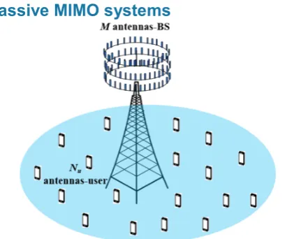
Figure 1. The downlink channel model in Massive
MIMO system
Let us consider a Massive MIMO system having the BS equipped with M antennas to simultaneously serve K users as illustrated in Fig. 1. Each user is equipped with Nu antennas. Thus, the
In addition, the Channel State Information (CSI) is assumed to be perfectly known by the BS. Among M
antennas, NT antennas is selected at a time for signal transmission, where NR ≤NT ≤M .
Let y∈�NR×1 be the overall received signal vector for
all users. Therefore, the relationship between the transmitted signal vector 1
1 2
[ T T... ]T T NR
K ×
= ∈
x x x x � and the
received signal vector y is represented by
y HWx n= + ,
(1) where H∈�N NR× T is channel matrix from selected
antennas at the BS to all K users, whose entries are assumed to be independent and identically distributed (i.i.d) random variables with zero mean and unit variance; [ 1 2... ] N NT R
K ×
= ∈
W W W W � is the
precoding matrix for all users; and NR1
u∈ ×
n �
is noise vector at the all users, whose entries are assumed to be i.i.d random variables with zero mean and variance σ2.
3. Transmit antenna groups selection
(TA-GS) algorithm in Massive MIMO
system
To balance the complexity and performance of the system, in this section, we propose the transmit antenna group selection algorithm based on the capacity analysis. The channel matrix from BS to all users is divided into G(G= NT / )δ groups, NR
g∈ ×δ
H � ,
(g=1,2,..., )G , where δ is a positive integer greater than 1. The channel matrix from BS to all users is expressed as
1 2
[ , ,..., ].
M = G
H H H H (2)
The first group, H1 includes δ first columns of the
channel matrix; the second group H2 includes the (δ + 1)th to the 2δth columns; and the last group, HG
includes the (M - δ)th to the Mth columns [13].
The first antenna group among G antenna groups, that has the largest channel capacity is selected by the following expression
{ }
1
(1, , )
2 (1, , )
argmax
argmaxlog det R ,
g G
H
N g g
g G T
g C g
N
r
∈
∈
=
= +
I H H
(3)
herein, Hg is the gthgroup of HM, g is the index of the
groups and ρ is the average signal-to-noise ratio (SNR) at the receiver side.
After the first antenna group is selected, we combine each of the remaining G - 1 antenna groups with
g
1 tocreate 1 1 2
[ , ]g g =[ g , g]∈ NR×δ
H H H � . The second antenna
group is selected such that the channel capacity provided by g1 and itself is maximized. It is expressed as follows
1
1
2 1
(1, , ),
2 (1, , ),
arg max { , }
arg max log det( )
g G g g
g G g g
g C g g
∈ ≠
∈ ≠
=
= Q
(4)
where R [ , ]1 [ , ]H1 N g g g g
T
N
r
= +
Q I H H . The same process is
carried out until NT transmit antennas are selected.
The proposed algorithm TA-GS is summarized in
Algorithm 1.
Algorithm 1: Proposed TA-GS algorithm
1.Input , , , , N MR
T R M
M N N δ H ∈� ×
2. Compute G NT
δ
= and create
1 2
[ , ,..., ]
M = G
H H H H .
3. Select the first antenna group according to:
1 2
(1, , )
argmaxlog det R H
N g g
g G T
g
N
r
∈
= +
I H H
.
4. Generate the channel matrix
H
[ , ,g1gk−1, ]g and selectthe kth antenna group according to:
1 1
2 (1, , ), , ,
arg max log det( )
k
k
g G g g g
g
−
∈ ≠
= Q
, where
1 1 1 1
[ , , k , ] [ , , k , ]
H g g− g g g− g
=
Q H H
5. Repeat Step 4 until NT transmit antennas are selected.
4. Proposed low-complexity lattice
reduction-aided linear group precoding
(LR-LGP).
4.1. Algorithm Analysis
In this Section, a linear group precoding algorithm based on the linear precoding algorithms combination with the ELR-SLV technique, called LR-LGP, is proposed. The precoding matrix for all user groups is given by
W=bW Wa b. (5) In the first step, the channel matrix H is divided
into L L( NR)
α
= groups (sub-matrices) NT
l∈ α×
H � ,
( 1,2,..., )l= L , where, α is a positive integer greater than 1. To be specific, the first group, H1, consists of the first row to the αth row of H; the second group, H2, is from
the (α+1)th row to the 2αth row; and the last group,
L
H , is from the (NR−α)th row to the NRth row.
Therefore, the channel matrix H can be rewritten as
1
2 .
L
=
H H H
H
(6)
In the second step, an MMSE weight matrix
T R
N N MMSE∈ ×
W � for all users is constructed as
follows
1 2
2 1
( )
, ,..., L ,
H H
MMSE n
GP GP GP MMSE MMSE MMSE
σ −
= +
=
W H HH I
W W W (7)
where 2 2/
n Es
σ =σ , Es is the symbol energy of the
transmitted signals, GPl NT
MMSE∈ ×α
W � , l=1,2, , L, are the
MMSE weight matrix for the lth user group. Applying QR decomposition to GPl
MMSE
W , we get
, l
GP
MMSE = l l
W Q R (8) where, N NT T
l∈ ×
Q � is a unitary matrix with orthogonal
columns, NT
l∈ ×α
R � is an upper triangular matrix. We
have
,1 ,1 ,2
,1 ,1,
l l l l l
l l
=
=
R
Q R Q Q
0 Q R
(9)
here l,1 NT
α ×
∈
Q � , Rl,1∈�α α× , ,2 NT (NT )
l
α × −
∈
Q � and the
zero matrix has size (NT −α α)× . Therefore, GPl ,1
a = l
W Q
is used as the precoding matrix for the lth user group. Using GPl,( 1, , )
a l= L
W , the first precoding matrix
T R
N N a∈ ×
W � is constructed as follows:
GP1, GP2,..., GPL .
a = a a a
W W W W (10)
In the next step, the second precoding matrix
R R
N N b∈ ×
W � in (5) is created by combining the linear
precoding algorithm and the lattice reduction technique to improve the quality of the system.
First, the effective channel matrix for the lth user group is generated as follows
GPl,
l = l a
H H W (11) which is then used to generate the extended matrix
2
ext l ∈ α α×
H � as follows
ext , R 2 .
l l s
N
E α
σ
=
H H I (12)
where Iα is a unit matrix size α α× .
Next, the channel matrix
( )
ext T lH is converted to the matrix Hˆl in the LR domain by using the ELR-SLV algorithm in [17] to give
ˆ T ext l = l l
H U H (13) where Ul is a unimodular matrix with integer elements
(det |Ul | 1)= . After that, the precoding matrix
l
GP b ∈ α α×
W � of the lth user group is designed as follows
GPl ˆH(ˆ ˆH)1
b = l l l l −
W A H H H (14)
where Al =
[
I 0α, α]
, 0α denotes the α α× zero matrix.Finally, the precoding matrix Wb is constructed using
,( 1, , ) l
GP
b l= L
W , as follows
1
2
0 0
0 0 .
0 0 L
GP b
GP b b
GP b
=
W W W
W
1
2
0 0
0 0
.
0 0
T T b
T L
=
U U U
U
(16)
The normalized power factor is defined as
(
)(
R)
H . a b a bN Tr
b =
W W W W
(17)
The proposed algorithm LR-LGP is summarized in
Algorithm 2.
Algorithm 2: The LR-LGP precoding algorithm
1.Input N NT, R,H
2. Decide the number of user groups L and compute the size of the sub-matrices.
3. Create the matrices H H H=[ ,1T T2,...,HT TL] and
1 , 2 ,..., L
GP GP GP MMSE = MMSE MMSE MMSE
W W W W .
4. Apply QR decomposition to GPl
MMSE
W , i.e.,
l
GP
MMSE = l l
W Q R for l=1, , L.
5. Create the weight matrices: GPl (:,1: )
a = l α
W Q for
1, ,
l= L.
6. Create the weight matrix Wa by arranging GPl
a
W as in equation (10).
7. Create the matrices GPl
l = l a
H H W and
2 ,
ext R
l l GP
s
N E
σ
=
H H I for l=1, , L.
8. Convert
( )
ext T lH into Hˆl, for l=1, , L, by applying
the ELR-SLV algorithm in [17].
9. Create the weight matrices GPl ˆH(ˆ ˆH) 1
b = l l l l −
W A H H H for
1, ,
l= L.
10. Create the weight matrix Wb by arranging GPl
b
W ,
1, ,
l= L, as in (15).
11. Output:
(
)(
R)
H a b a bN Tr
b =
W W W W
and
a b
b
=
W W W .
The received signal vector for all users is given by
y HWx n= + . (18)
Using y in (18), the transmit signal vector is estimated as follows
1 1
1
ˆ b Qz α bz( )b L bz( )b L ,
α b − −
= + −
y
x U U 1 U 1 (19)
herein α=1/ 2, 1(1 )
2
z m j
b = − + , m is the number of
bits in a transmitted symbol, NR 1
L∈R ×
1 is a column vector containing NR ones. Qz[.] represents the rounding operation. From (18) and (19), it follows that:
ˆ 2 1 . 2
b zQ b
= +
n
x x U (20)
0.35 0.4 0.45 0.5 0.55
1/beta 0
0.1 0.2 0.3 0.4 0.5 0.6 0.7 0.8 0.9 1
ECDF
LC-RBD-LR-ZF
LR-LGP with L=4, 60 60 no selec LR-LGP with L=6, 60 60 no selec LR-LGP with L=10, 60 60 no selec
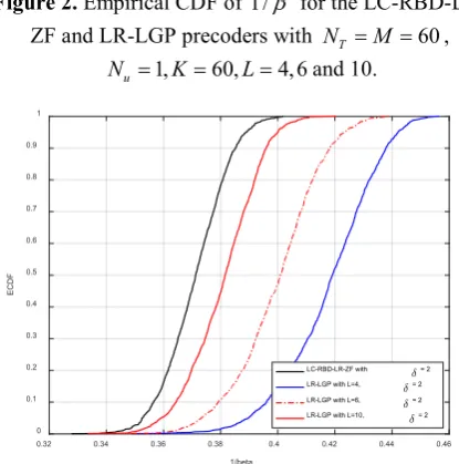
Figure 2. Empirical CDF of 1/b for the
LC-RBD-LR-ZF and LR-LGP precoders with NT =M =60, 1, 60, 4,6
u
N = K= L= and 10.
0.32 0.34 0.36 0.38 0.4 0.42 0.44 0.46 1/beta
0 0.1 0.2 0.3 0.4 0.5 0.6 0.7 0.8 0.9 1
ECDF
LC-RBD-LR-ZF with = 2 LR-LGP with L=4, = 2 LR-LGP with L=6, = 2 LR-LGP with L=10, = 2
Figure 3. Empirical CDF of 1/b for the
LC-RBD-LR-ZF and LR-LGP precoders with M =90,NT =60, 1, 60, 4,6
u
From (20), we can see that x is correctly recovered if 1
2
z
Q b=
n 0. This means that for a given noise power,
the component 1/b will be the factor that determines the system performance. In Fig. 2 and Fig. 3, the empirical cumulative distribution functions (ECDFs) of the 1/b in (20) are shown for the LC-RBD-LR-ZF and LR-LGP precoders when the system is with and without transmit antenna selection. For the same system configuration, the simulation results show that the LC-RBD-LR-ZF precoder generates smaller 1/b than the LR-LGP precoder. This means that the LC-RBD-LR-ZF precoder will probably outperform the LR-LGP precoder for the same system configuration. Moreover, the more sub-groups are generated the smaller 1/b
becomes, and hence the better system performance can be achieved. It can also be observed from the two figures that the transmit antenna selection technique allows the system to reduce 1/b , thereby improving the system performance.
4.2. Computational Complexity Analysis
In this sub section, we evaluate the computational complexity of the proposed LR-LGP algorithm and the LC-RBD-LR-ZF algorithm in [12]. The complexities are evaluated by counting the required floating point operations (flops). We assume that each real operation (an addition, a multiplication or a division) is counted as a flop. Hence, a complex multiplication and a division equal to 6 flops and 11 flops, respectively. It is worth noting that the QR decomposition of an r t×
complex matrix requires 6rt2+4rt t− −2 t flops.
Based on the above assumptions, the computational complexities of the proposed LR-LGP algorithm and the LC-RBD-LR-ZF one are computed in details as follows
a. Complexity of the LC-RBD-LR-ZF algorithm
The computational complexity of the LC-RBD-LR-ZF algorithm is given by:
( ).
a b c
F F F F= + + flops (21)
herein Fa and Fb are the number of flops to calculate
a
P and Pb, respectively.
c
F is the number of flops of the multiplication two matrices Pa and Pb. Fa and Fb
are evaluated and expressed in the (22) and (23).
]
2
2
6( )( )
4( )( ) ( )
( ) ( )
a R u R T u
R u R T u R T u R T u
F K N N N N N
N N N N N N N N
N N N flops
= − + −
+ − + − − + −
− + −
(22)
2 2
3 2 3 2
2
(8 2 ) (16 2
8 2 ) (8 16
2 2 ) ( )
T u T u u T u T u u update LLL u u T
u u T b
F K N N N N K N N N N
N N F K N N N
N N N flops
−
− + −
+ − + + +
− −
=
(23)
Note that in (23), Fupdate LLL− is the computational
cost of the update operation for the LLL technique, which is obtained by computer simulation.
c
F is evaluated to be
2
8 2 ( ).
c T R T R
F = KN N − N N flops (24) From (21)-(24), the total number of flops of the LC-RBD-LR-ZF algorithm is obtained as in (25).
]
2
2
2
2 3 2
3 2 2
2
4
6( )( )
4( )( ) ( )
( ) (8 2 )
(16 2 8 2 )
(8 16 2 2 )
8 2 ( )
~ ( )
R u R T u
R u R T u R T u R T u T u T u
u T u T u u update LLL
u u T u u T T R T R
R
F K N N N N N
N N N N N N N N
N N N K N N N N
K N N N N N N F
K N N N N N N
KN N N N flops
O N
−
= − + −
+ − + − − + −
− + − −
+ − + − + + + − −
+
− +
(25)
b. Complexity of the LR-LGP algorithm
The computational complexity of the proposed LR-LGP algorithm is given by
1 A B C ( ).
F F= +F +F flops (26) where FA and FB are the number of flops to calculate
a
W and Wb, respectively. FC is the number of flops of multiplying the two matrices Wa and Wb.
A
F is expressed as
( ),
A MMSE QR
F =F +F flops (27)
where FMMSE is the number of flops to compute the
MMSE
decomposition operations. FMMSE and FQR are calculated
as follows
3 2 2
8 16
2 1 ( ).
MMSE R R T R R T R
F N N N N
N N N flops
= + −
− + + (28)
2 2
(6 4 ) ( ).
QR T T
F =L N α+ N α α− −α flops (29) Therefore, the total number of flops to find Wa is given by
3 2 2
2 2
8 16 2
1 (6 4 ) ( ).
A MMSE QR
R R T R R T R
T T
F F F
N N N N N N N
L N α N α α α flops
= +
= + − − +
+ + + − −
(30)
B
F is calculated as follows
2 3 4 ( ),
B
F =F F F+ + flops (31)
where F2, F3 and F4 are the total number of flops to
compute Hl, Hˆl and WbGPl matrices, respectively. F2
and F3 are computed as
2 2
2 (8 T 2 ) ( ).
F =L N α − α flops (32)
3 5 6 update SLV ( ).
F =F F F+ + − flops (33)
herein F5 and F6 are the number of flops to compute
( )
{
T}
H( )
T 1ext ext
l l
−
=
C H H and ˆ T ext
l = l l
H U H ,
respectively. Fupdate SLV− is computational cost of the
ELR-SLV algorithm's update operations, which is obtained by computer simulation. Therefore, F3 is calculated as
3 2 3 2
3 (24 2 ) (16 4 )
( ).
update SLV
F L L
LF flops
α α α α
−
= − + −
+ (34)
The number of flops to find all GPl
b
W matrices is given by
3 2
4 (56 8 ) ( ).
F =L α − α flops (35)
Hence, the total number of flops to find the precoding matrix Wb is represented by
2 2 3 2 3
2 3 2
(8 2 ) (24 2 ) (16
4 ) (56 8 )( ).
B T
update SLV
F L N L L
LF L flops
α α α α α
α − α α
− + − +
− + + −
=
(36)
C
F is calculated by
2 2
8 2 ( ).
C R T R
F = N N − N flops (37)
From the above analysis results, the total number of flops for the LR-LGP algorithm is given in the (38)
3 2 2
1
2 2 2 2
3 2 3 2
3 2 2 2
3
8 16 2 1
(6 4 ) (8 2 )
(24 2 ) (16 4 )
(56 8 ) 8 2 ( ).
~ ( )
R R T R R T R
T T T
update SLV
R T R R
F N N N N N N N
L N N L N
L L LF
L N N N flops
O N
α α α α α α
α α α α
α α
−
+ − − + +
+ + − − + −
+ −
− + −
+
+ − +
=
(38)
5. Simulation results
In this section, we evaluate and compare not only the BER performance but also the computational complexity of the LR-LGP precoder with those of the LC-RBD-LR-ZF precoder in [12]. The channel between the BS and all users are assumed to be semi-static Rayleigh fading.
0 5 10 15 20 25 30
SNR [dB] 10-4
10-3 10-2 10-1 100
BER
LC-RBD-LR-ZF LR-LGP with L=4 LR-LGP with L=6 LR-LGP with L=10
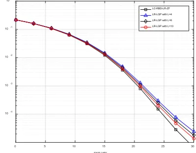
Figure 4. The system performance with NT =M =60,
1, 60, 4,6,10.
u
N = K = L=
Fig. 4 illustrates the system performance for the proposed algorithm LR-LGP and the LC-RBD-LR-ZF algorithm in [12]. The simulation parameters are as follows: NT =M =60, Nu =1,K=60 and 4-QAM modulation. The number of user groups for the LR-LGP precoder is L = 4; 6, and 10. The simulation results in Fig. 4 show that the BER performance of the proposed algorithm LR-LGP is asymptotic to the LC-RBD-LR-ZF algorithm when L increases. Specifically, at BER 10= −3 the proposed algorithm suffers from
is significantly lower than the LC-RBD-LR-ZF algorithm, as confirmed by the simulation results in Fig. 7.
Fig. 5 and Fig. 6 illustrate the system performance when the TA-GS technique is applied. To get the results, the following parameters are used: M =90,
60
T
N = ,Nu =1,K=60,L=4,6,10, 4-QAM modulation,
2
δ = for Fig. 5 and δ =3 for Fig. 6. It can be seen from the figures that the system performance is significantly improved as the TA-GS technique is adopted. Specifically, at BER 10= −3 for the same precoder, the
system performance improves by about 2 dB and 1.5 dB in SNR corresponding to δ =2 and δ =3 when compared to the case of no antenna selection. Besides, Fig. 5 and Fig. 6 show that the performance improvement is inversely proportional to δ .
0 5 10 15 20 25 30
SNR [dB] 10-4
10-3
10-2 10-1 100
BER
LR-LGP with L=4, = 2 LR-LGP with L=6, = 2 LR-LGP with L=10, = 2 LC-RBD-LR-ZF = 2 LR-LGP with L=4, 60 60 no selec LR-LGP with L=6, 60 60 no selec LR-LGP with L=10, 60 60 no selec LC-RBD-LR-ZF, 60 60 no selec
Figure 5. The system performance with M =90,
60
T
N = , Nu =1,K=60,L=4,6,10,δ =2
0 5 10 15 20 25 30
SNR [dB] 10-4
10-3 10-2
10-1
100
BER
LR-LGP with L=4, = 3 LR-LGP with L=6, = 3 LR-LGP with L=10, = 3 LC-RBD-LR-Z, = 3 LR-LGP with L=4, 60 60 no selec LR-LGP with L=6, 60 60 no selec LR-LGP with L=10, 60 60 no selec LC-RBD-LR-ZF, 60 60 no selec
Figure 6. The system performance with M =90,
60
T
N = , Nu =1,K =60,L=4,6,10,δ =3
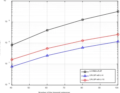
Fig. 7 illustrate the computational complexities of the proposed algorithm LR-LGP and the LC-RBD-LR-ZF algorithm. In this scenario, NT is varied from 40 to 100 transmit antennas, NR =NT , L = 4 and L = 10. It can be
seen from the figure that the computational complexities of the proposed precoder is noticeably lower than those of the LC-RBD-LR-ZF precoder. Specifically, at NT = 80 antennas, the computational complexities of the LR-LGP precoder with L = 4 and L = 10 groups are equal to about 6.25%, 13.54% of the LC-RBD-LR-ZF precoder’s complexity, respectively. We can also see from the figure that the computational complexity of the LR-LGP precoder increases as the number of groups L increases.
40 50 60 70 80 90 100
Number of the transmit antennas 106
107
108
109
1010
Number of flops
LC-RBD-LR-ZF LR-LGP with L=4 LR-LGP with L=10
Figure 7. Compare the complexity of the proposed
precoding algorithm and the LC-RBD-LR-ZF algorithm in [12]
6. Conclusions
the system performance significantly improves when applying the transmit selection technique. Simulation results also show that the system performance inversely proportional to δ. Furthermore, the LR-LGP precoder has remarkably lower complexity than the LC-RBD-LR-ZF, whereas its BER performance approaches that of the LC-RBD-LR-ZF precoder when L increases. As a consequence, the LR-LGP can be a potential candidate for signal beamforming at the BS of Massive MIMO systems.
Acknowledgement:
This paper has been presented in part at International Conference on Advanced Technologies for Communications, ATC, 2018References
[1] H. Q. Ngo, Massive MIMO: Fundamentals and system
designs. Linkoping University Electronic Press, 2015, vol. 1642
[2] Q. H. Spencer, C. B. Peel, A. L. Swindlehurst, and M.
Haardt, “An introduction to the multi-user mimo
downlink,” IEEE Communications Magazine, vol. 42, no.
10, pp. 60–67, Oct 2004.
[3] L. Lu, G. Y. Li, A. L. Swindlehurst, A. Ashikhmin, and
R. Zhang, “An overview of massive mimo: Benefits and
challenges,” IEEE Journal of Selected Topics in Signal
Processing, vol. 8, no. 5, pp. 742–758, Oct 2014
[4] T. L. Marzetta, “Noncooperative cellular wireless with
unlimited numbers of base station antennas,” IEEE
Transactions on Wireless Communications, vol. 9, no. 11, pp. 3590–3600, November 2010.
[5] ——, “Massive mimo: An introduction,” Bell Labs
Technical Journal, vol. 20, pp. 11–22, 2015.
[6] H. Y. T. L. Marzetta, E. G. Larsson and H. Q. Ngo,
Fundamentals of Massive MIMO. Cambridge University Press, 2016.
[7] E. G. Larsson, O. Edfors, F. Tufvesson, and T. L.
Marzetta, “Massive mimo for next generation wireless
systems,” IEEE Communications Magazine, vol. 52, no. 2,
pp. 186–195, February 2014.
[8] V. P. Selvan, M. S. Iqbal, and H. S. Al-Raweshidy,
“Performance analysis of linear precoding schemes for
very large multi-user mimo downlink system,” Fourth
edition of the International Conference on the Innovative Computing Technology (INTECH 2014), pp. 219–224, Aug
2014.
[9] H. Q. Ngo, E. G. Larsson, and T. L. Marzetta, “Massive
mu-mimo downlink tdd systems with linear precoding and downlink pilots,” pp. 293–298, 2013.
[10]Y. S. Cho, J. Kim, W. Y. Yang, and C. G. Kang,
MIMO-OFDM wireless communications with MATLAB. John Wiley & Sons, 2010.
[11]M. . Simarro, F. Domene, F. J. Martínez-Zaldívar, and
A. Gonzalez, “Block diagonalization aided precoding
algorithm for large mu-mimo systems,” 2017 13th
International Wireless Communications and Mobile
Computing Conference (IWCMC), pp. 576–581, June 2017.
[12]K. Zu and R. C. d. Lamare, “Low-complexity lattice
reductionaided regularized block diagonalization for
mu-mimo systems,” IEEE Communications Letters, vol. 16,
no. 6, pp. 925–928, June 2012.
[13]V. K. Dinh, M. Tuan Le, V. D. Ngo, and C. Hieu Ta,
“Transmit antenna selection by group combination
precoding in massive mimo system,” 2018 International
Conference on Advanced Technologies for Communications (ATC), pp. 276–281, Oct 2018.
[14]W. S. Bing Fang, Zuping Qian and W. Zhong, “Raise: A
new fast transmit antenna selection algorithm for massive
mimo systems,” Springer Science+Business Media New
York, September 2014.
[15]T. Tai, W. Chung, and T. Lee, “A low complexity antenna
selection algorithm for energy efficiency in massive mimo
systems,” 2015 IEEE International Conference on Data
Science and Data Intensive Systems, pp. 284–289, Dec 2015.
[16]M. T. A. Rana, R. Vesilo, and I. B. Collings, “Antenna
selection in massive mimo using non-central principal
component analysis,” 2016 26th International
Telecommunication Networks and Applications Conference (ITNAC), pp. 283–288, Dec 2016.
[17]Q. Zhou and X. Ma, “Element-based lattice reduction
algorithms for large mimo detection,” IEEE Journal on