Early Stage Software Effort Estimation using Random Forest
Technique based on Optimized Class Point Approach
SHASHANKMOULISATAPATHY1
BARADAPRASANNAACHARYA2
SANTANUKUMARRATH3
Department of Computer Science and Engineering National Institute of Technology, Rourkela
Rourkela - 769008, Odisha, India
1
2
3
Abstract. Evaluating software development effort remains a complex issue drawing in extensive re-search consideration. The success of software development depends very much on proper estimation of effort required to develop the software. Hence, correctly assessing the effort needed to develop a soft-ware product is a major concern in softsoft-ware industries. Random Forest (RF) technique is prevalently utilized machine learning techniques that aides in getting enhanced evaluated values. The main research work carried out in this paper is to accurately estimate the effort required in developing various software projects by using the optimized class point approach (CPA). Then, optimization of the effort parameters is achieved using the RF technique to obtain better prediction accuracy. Furthermore, performance com-parisons of the models obtained using the RF technique with other machine learning techniques such as the Multi-Layer Perceptron (MLP), Radial Basis Function Network (RBFN), Support Vector Regres-sion (SVR) and Stochastic Gradient Boosting (SGB) techniques are presented in order to highlight the performance achieved by each technique.
Keywords: Class Point Approach, Object Oriented Analysis and Design, Random Forest, Software Effort Estimation.
(Received September 11th, 2014 / Accepted January 20th, 2015)
1 Introduction
Object-oriented (OO) technology is the accepted methodology for software development in major indus-tries. Various features are offered by object oriented programming concepts, which play an important role during software development process [3]. With the in-crease in the complexities associated with modern day software projects, the need for early and accurate ef-fort estimation in the software development phase has become pivotal. Currently used effort estimation tech-niques like Function Point (FP) and COCOMO, fail to consistently estimate the cost and effort required to
de-velop the software [20]. These techniques are not ca-pable of measuring cost and effort because they are tailored for procedural-oriented software development paradigm [12, 21]. The procedural oriented paradigm and object-oriented paradigm differ because the former splits the data and procedure; while the latter combines them.
depends upon accurate effort estimation. Since class is the fundamental logical unit of an OO system, the utilization of the class point methodology to compute the project effort serves to get a improved result. Dur-ing the calculation procedure of the final adjusted class point, two measures, CP1 and CP2, are utilized. CP1 is figured utilizing two measures, Number of External Methods (NEM) and Number of Services Requested (NSR); whereas CP2 is ascertained by utilizing an al-ternate metric as a part of expansion to NEM and NSR, Number of Attributes (NOA). NEM figures the mea-sure of the interface of a class and is directed by the measure of local public methods, although NSR gives a measure of the linkage of the components of the soft-ware system. On the other hand, NOA helps in finding out the number of attributes utilized in a class. In case of function point approach (FPA) and CPA, the Techni-cal Complexity Factor (TCF) is Techni-calculated based on the impact of various general characteristics of a system. However, in both these cases, the non-technical fac-tors such as effectiveness of the management, technical competence of developers, security of the system, sys-tem’s reliability, syssys-tem’s maintenance capability and system’s portability are not looked into [25]. Hence in this study, the optimized CPA is utilized to ascertain the effort needed to create the software adopting these six non-technical factors. The fuzzy logic approach is used to optimize the complexity value of various types of class which in-turn optimizes the final estimated class point value. Likewise with a specific end goal to ac-complish better prediction accuracy, a Random Forest (RF)-based effort estimation model is applied over the obtained optimized class point value. The results ob-tained from the RF-based estimation model are then compared with the results obtained from other machine learning techniques i.e., MLP, RBFN, SVR and SGB-based models in order to access their performance. Re-sults proved that the RF technique-based software effort estimation model outperforms other models.
2 Related Work
Costagliola et al. [5] observed that the prediction ac-curacy of CP1 and CP2 under the class point approach were 75% and 83% respectively. They drew this con-clusion by conducting an experiment on a dataset with forty projects. Zhou and Liu [25] extended this method-ology by including an alternate measure CP3 and con-sidered twenty four attributes rather than the eighteen acknowledged by Gennaro Costagliola et al. By uti-lizing this methodology, they watched that the perfor-mance of CP1 and CP2 stay unaltered, although the number of characteristics changed. Kanmani et al. [9]
utilized the same CPA with the ANN model for map-ping CP1 and CP2 into the assessed software devel-opment effort and observed that the prediction accu-racy for CP1 was enhanced to 83% and CP2 to 87%. Kim et al. [11] presented some new meanings of class point to interpret system’s architectural complexity in an improved way. They utilized various additional pa-rameters along with NEM, NSR and NOA to compute the total number of adjusted class point value. Kan-mani et al. [10] introduced a novel technique to utilize the CPA with fuzzy logic by embracing the subtrac-tive clustering technique for computing effort and con-trasted it with the result acquired from the ANN. They observed that the fuzzy system focused around the sub-tractive clustering technique outperforms ANN. Sheta [23] used Takagi-Sugeno-Kang (TSK) fuzzy model to develop fuzzy models for two different type of nonlin-ear processes. The first one is NASA software projects effort estimation process and the second one is the stock market prediction process for S& P 500.
Satapathy et al. [22] proposed a novel SVR based effort estimation technique-based class point approach and obtain promising results. Satapathy et al. [19] also proposed a novel SGB technique-based effort estima-tion model using class point approach. From the anal-ysis, it is observed that the SGB technique-based effort estimation model provides improved prediction accu-racy than MLP and RBFN technique. Elish [6] used multiple additive regression trees as a novel advanced data mining technique that broadens and enhances the classification and regression trees (CART) model using a treeboost technique. The predicted results obtained were then compared with linear regression, RBFN, and SVR models with the help of a NASA software project data set and found an improved estimation accuracy. Nassif et al. [17] presented a novel regression model for software effort estimation focused around use case dia-grams. By analyzing the outcome, they proved that the the software effort estimation accuracy can be improved by 16.5% using PRED(25) and 25% using PRED(35). Elyassami et al. [7] investigate the utilization of Fuzzy choice tree for software effort estimation. The proposed model empower to handle questionable and loose in-formation, which enhance the correctness of obtained evaluations.
UCP model with the assistance of 240 data and ob-tained an improved result than other regression models. Pahariya et al. [18] proposed a new concurrent archi-tecture for a genetic programming based feature selec-tion algorithm for software effort estimaselec-tion and com-pared the predicted effort with other computational in-telligence techniques. The results show that the new recurrent architecture design for GA performs better than the other models. Nassif et al. [14] also proposed some other techniques using fuzzy logic and ANN to enhance the correctness of the UCP model and achieved up to 22% improvement in prediction accuracy result.. Huang et al. [8] proposed a neuro-fuzzy technique for software effort estimation and obtained promising re-sults. Baskeles et al. [1] proposed a model that uses machine learning techniques and assess the model us-ing the data collected from public data sets and the data collected from software industries. From investigation, it is discovered that the utilization of any one model can’t create the best comes about for software effort es-timation.
3 Methodologies Used
The following methodologies are used in this paper to calculate the effort of a software product.
3.1 Class Point Approach (CPA)
The CPA was presented by Gennaro Costagliola et al. in 1998 [4]. It was focused around the FPA methodol-ogy to speak to the interior qualities of a software. The essential thought of the CPA system is calculation of classes in a project. It is determined from the percep-tion that in the procedural model funcpercep-tions or methods are the essential programming units; while, in the OO model, classes are the coherent building pieces.
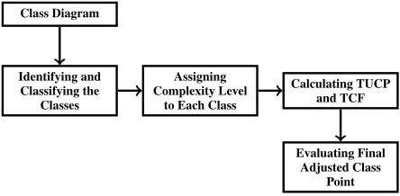
The block diagram, demonstrated in figure 1, states the steps to compute the project development effort us-ing class point approach.
Class Diagram
Identifying and Classifying the
Classes
Assigning Complexity Level
to Each Class
Calculating TUCP and TCF
Evaluating Final Adjusted Class
Point
Figure 1:Final Adjusted Class Point Calculation Steps
The system to acquire the amount of class points is isolated into three principle stages [5].
• Estimating information processing size
– Identifying and classifying the classes
– Assigning complexity level for each classi-fied class
– Calculating the Total Unadjusted Class Points (TUCP) value
• Estimating the Technical Complexity Factor (TCF) value
• Calculating the final value of Adjusted Class Point (CP)
In this study, the above phases are followed to cal-culate final optimized class points. Detailed descrip-tions of all the phases were already provided by Gen-naro Costagliola et al. [5]. Herein, the total number of optimized class point value is then used as an input pa-rameter to the random forest model to calculate the es-timated effort.
3.1.1 Fuzzy Logic System
Fuzzy sets were presented by L. A. Zadeh (1965) as a method for speaking to and controlling information that was not exact, but instead fuzzy. Fuzzy logic gives a derivation morphology that empowers rough human thinking capacities to be connected to infor-mation based frameworks [21]. Fuzzy system com-prises of three principle segments:fuzzification process, derivation from fuzzy rulesanddefuzzification process. Among different fuzzy models, the model presented by Takagi, Sugeno and Kang (TSK fuzzy) [24] is more ap-plicable for sample data based fuzzy modeling, on the grounds that it requires less rules. Each rule’s outcome with linear function can portray the information yield mapping in a vast reach, and the fuzzy implications uti-lized within the model is likewise basic. In this study, fuzzy modeling has been utilized to improve the com-plexity of TUCP and fuzzy subtractive clustering to es-timate the effort.
3.2 Random Forest Technique
tree models, ensemble model combines the results from different models of similar type or different types.
The concept behind it is that random forests grow many classification trees. To generate many classifi-cation trees, a random vectorλand an input vectorx
is used. A random vector λk is produced for thekth
tree, which is autonomous of the previous random vec-tors λ1, ..., λk−1, however with the equal distribution.
A tree is developed utilizing the training set and λk,
which generates a classifierh(x, λk) wherexis an
in-put vector. To categorize new object from an inin-put vec-tor, the input vectorxis put down each of the trees in the forest. Each tree provides a classification by voting for that class. Then, the classification having the max-imum number of votes among over all the trees in the forest is chosen. In case of regression, the prediction accuracy of the forest is obtained by taking the average of the individual tree predictions.
RF for regression purpose are created by developing trees relying upon a random vectorλspecified that the tree predictorh(x, λ) undertakes numerical data instead of class labels. The output produced by the predictor is
h(x)and the actual effort value isY. For any numerical predictor h(x), the generalized mean-squared error is calculated as
Ex,Y(Y −h(x))2 (1)
By calculating the average value obtained overktrees
h(x, λk), the RF predictor is modeled.
4 Proposed Approach
The proposed approach is applied over forty data set used in [5]. The utilization of such data set proposes to assess software development effort and provides intro-ductory test evidence of the viability of the CPA. The utilization of this data set helps to evaluate the effort required to develop software and validate the practica-bility of improvement. In the data set, every row dis-plays the details of one project developed in JAVA lan-guage, indicating values of NEM, NSR and NOA for that project. Apart from that, it also displays values of CP1, CP2 and the actual effort (denoted by EFH) ex-pressed in terms of person-hours required to success-fully complete the project.These data are utilized to de-velop the random forest technique based software effort estimation model.
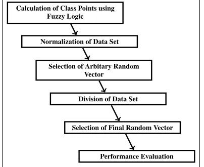
The diagram demonstrated in figure 2 displays the proposed steps used to determine the predicted effort using the random forest technique-based on optimized class point approach.
To compute the software development effort, essen-tially the accompanying steps are utilized.
Calculation of Class Points using Fuzzy Logic
Normalization of Data Set
Selection of Arbitary Random Vector
Division of Data Set
Selection of Final Random Vector
Performance Evaluation
Figure 2:Proposed Steps Used for Effort Estimation using Random
Forest Technique
Proposed Steps for Software Effort Estimation
1. Calculation of Class Points using Fuzzy Logic: After collecting the data from other developed projects, the CP2 value is calculated from the UML diagram. This generated CP2 value is used as an input argument. But in this study, fuzzy modeling technique has been used to calculate the weights of the various types of classes to get more accurate TUCP value. Here atriangular member-ship function is used to define their membership and compute their weights.
2. Normalization of Dataset: Input parameter val-ues are normalized within the range 0 to 1. LetS represents the complete dataset andsrepresents a record in theS. Then the normalized value ofsis obtained by using the following formula :
N ormalized(s) = s−min(S)
max(S)−min(S) (2)
where
min(S)= min value inS.
max(S)= max value inS.
ifmin(S)is same asmax(S), then Normalized(s) value is assigned as 0.5.
3. Selection of Arbitrary Random Vector: Random forest have randomness in input data and in split-ting at nodes . Hence, initially an arbitrary random vector is selected to provide randomness in input data and to start the implementation process. 4. Division of dataset: Total no. of data are divided
5. Selection of Final Random Vector: Prediction re-sults vary according to random vector. So an eval-uation function(1- MMRE + Prediction Accuracy) is used to find a random vector. The random vec-tor, which provides optimum value for the evalua-tion funcevalua-tion is considered as final random vector.
6. Performance Evaluation: In this study, the Mean Magnitude of Relative Error (MMRE) and the Pre-diction Accuracy (PRED) are the two measures used to evaluate the performance of the model for test samples. Results obtained from proposed model are then compared with existing results to access its performance accuracy.
The above steps are followed to implement the ran-dom forest technique based effort estimation model. Finally, a comparisons of results obtained using the random forest technique based effort estimation model with the results obtained from the MLP, RBFN, SVR and SGB techniques-based models are presented to as-sess their performances.
5 Experimental Details
In this study, for implementing the proposed approach, dataset having forty data is being used which is also used by G. Costagliola et al. [5]. The detail descrip-tion about the data set has already been provided in proposed approach section. After computing the no. of class points, the dataset is then scaled. The scaled dataset is split into two subsets i.e.,training setandtest set. Thetraining setis used for learning reason; though thetest set is used only for assessing the exactness of prediction of the trained model.
5.1 Calculating Class Complexity Value Using
Fuzzy Logic
In the figuring of CP, Mamdani-type FIS is utilized in light of the fact that Mamdani-type FIS technique is broadly acknowledged for catching expert knowledge. It permits us to depict the expertise in more natural and human-like way. On the other hand, Mamdani-type FIS involves a significant computational load. The model has two inputs i.e. NEM and NOA; and one yield i.e. CP as demonstrated in figure 3. The primary procedures of this system incorporate four exercises: fuzzification, fuzzy rule base, fuzzy inference engine and defuzzifica-tion. All the input variables in this model are changed to the fuzzy variables focused around the fuzzification process. The complexity levels, for example, Low, Av-erage, High, and Very High are characterized for NOA
and NEM variables, for diverse number of services re-quested (NSR). The steps to compute the class point utilizing FIS is given below.
1. Initially develop the UML diagrams of a project and identify the number of classes in it.
2. This step deals with classification of each class into various domain such as PDT/HIT/DMT/TMT. 3. In this step, various parameters such as no. of ex-ternal methods (NEM), no. of services requested (NSR) and no. of attributes (NOA) need to be ex-tracted from UML diagram.
4. Then the complexity level such as Low, Average, High and Very High is assigned to each class fo-cusing around their obtained NEM, NSR and NOA value.
5. During this step, the numeric value of complexity level assigned to a class is found out using fuzzy logic technique.
6. Then the Unadjusted Class Point (UACP) is calcu-lated by multiplying the numeric value obtained in Step-5.
7. Then the TUCP is calculated by adding the UACP of all classes.
8. This step deals with calculating TCF value by us-ing twenty four general system characteristics. 9. Finally, the adjusted CP count is calculated by
multiplying TUCP with TCF.
5.1.1 Results and Discussion
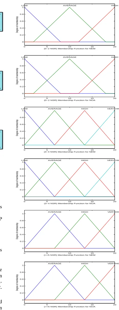
A fuzzy set is defined for each linguistic value with a Triangular Membership Function (TRIMF), in figure 4. The fuzzy sets corresponding to the various associated linguistic values is defined for each type of inputs.
The proposed fuzzy guidelines hold the linguistic variables identified with the project. It is vital to note that these rules were balanced or adjusted, and in addition all pertinence level functions, as per the tests and the aspects of the project. The amount of principles those have been utilized as a part of model are 9, 16, and 9 for (0-2) NSR, (3-4) NSR and (≥5) NSR separately for all input variables.
Fuzzy rules for (0-2)NSR:
System CP (NSR 0−2): 2 inputs, 1 outputs, 9 rules NEM (3)
NOA (3)
CP (3) CP (NSR 0−2)
(mamdani)
9 rules
System CP (NSR 3−4): 2 inputs, 1 outputs, 16 rules NEM (4)
NOA (4)
CP (4) CP (NSR 3−4)
(mamdani)
16 rules
System CP (NSR>=5): 2 inputs, 1 outputs, 9 rules NEM (3)
NOA (3)
CP (3) CP (NSR>=5)
(mamdani)
9 rules
Figure 3:FIS for Class Point Calculation
LOW.
If NEM is LOW and NOA is HIGH THEN CP is AVERAGE.
If NEM is LOW and NOA is AVRERAGE THEN CP is AVRERAGE.
. . .
If NEM is HIGH and NOA is HIGH THEN CP is HIGH.
The MATLAB FIS was utilized as a part of the fuzzy computations, notwithstanding the Max-Min composition operator, the Mandani implication opera-tor, and the Maximum operator for aggregation and af-ter that the model is defuzzified.
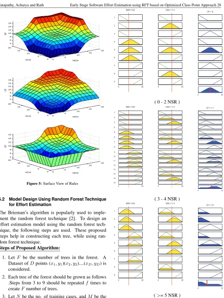
Figure 5 shows the output surface of the FIS utilized for CP estimation. The fuzzy rule viewer indicated in figure 6 serves to ascertain the whole implication pro-cess from starting to end.
0 5 10 15 20
0 0.2 0.4 0.6 0.8 1
(0−2 NSR) Membership Function for NEM
Degree of membership
LOW AVERAGE HIGH
0 5 10 15 20
0 0.2 0.4 0.6 0.8 1
(0−2 NSR) Membership Function for NOA
Degree of membership
LOW AVERAGE HIGH
0 5 10 15 20
0 0.2 0.4 0.6 0.8 1
(3−4 NSR) Membership Function for NEM
Degree of membership
LOW AVERAGE HIGH VERY HIGH
0 5 10 15 20
0 0.2 0.4 0.6 0.8 1
(3−4 NSR) Membership Function for NOA
Degree of membership
LOW AVERAGE HIGH VERY HIGH
0 5 10 15 20
0 0.2 0.4 0.6 0.8 1
(>=5 NSR) Membership Function for NEM
Degree of membership
AVERAGE HIGH VERYHIGH
0 5 10 15 20
0 0.2 0.4 0.6 0.8 1
(>=5 NSR) Membership Function for NOA
Degree of membership
AVERAGE HIGH VERYHIGH
0 5
10 15
20
0 5 10 15 20
4 6 8 10 12 14 16
NEM NOA
CP
0 5
10 15
20
0 5 10 15 20
4 6 8 10 12 14 16
NEM NOA
CP
0 5
10 15
20
0 5 10 15 20
4 6 8 10 12 14 16
NEM NOA
CP
Figure 5:Surface View of Rules
5.2 Model Design Using Random Forest Technique for Effort Estimation
The Brieman’s algorithm is popularly used to imple-ment the random forest technique [2]. To design an effort estimation model using the random forest tech-nique, the following steps are used. These proposed steps help in constructing each tree, while using ran-dom forest technique.
Steps of Proposed Algorithm:
1. Let F be the number of trees in the forest. A Dataset ofDpoints (x1, y1)(x2, y2)....(xD, yD) is
considered.
2. Each tree of the forest should be grown as follows .Steps from 3 to 9 should be repeatedf times to createFnumber of trees.
3. LetN be the no. of training cases, andM be the no. of variables in the classifier.
4. To select training set for the tree, a random sample ofncases - yet with substitution, from the original
1
CP = 10
2
3
4
5
6
7
8
9
0 20 0 20
NEM = 8.53 NOA = 11.4
0 20
( 0 - 2 NSR )
1
CP = 11.1
2
3
4
5
6
7 8
9
NEM = 8.53 NOA = 11.4
9 10 11 12 13 14 15 16
0 20 0 20
0 20
( 3 - 4 NSR )
1
CP = 7.31
2
3
4
5
6
7
8
9
0 20 0 20
NEM = 8.53 NOA = 11.4
0 20
(>= 5 NSR )
data of allN accessible training cases is choosen. Whatever is left of the cases are utilized to evaluate the error of the tree, by foreseeing their classes. 5. A RF treeTf is developed to the loaded data, by
repeatedly rehashing the accompanying steps for every terminal node of the tree, till the minimum node sizenminis arrived. Keeping in mind the end
goal to make more randomness, distinctive dataset for each one trees is made.
6. The no. of input variablesmis selected to ascer-tain the choice at a tree node. The value ofmought to be substantially short of whatM.
7. For each tree node,mnumber of variables should be randomly chosen on which the decision at that node is based.
8. The best split focused around thesemvariables in the training set is calculated. The value ofmought to be held consistent throughout the development of the forest. Each tree should be fully grown and not pruned.
9. Then, the results of ensemble of trees
T1, T2, ..., Tf, ...., TFare collected.
10. The input vector should be put down for each of the trees in the forest. In regression, it is the aver-age of the individual tree predictions.
YF(x) = 1/F
F
X
f=1
Tf(x) (3)
where
YF(x)is the predicted value for the input
vectorx.
T1(x), T2(x), ..., Tf(x) represents
predic-tion value of individual trees.
There are various data objects generated by random for-est technique, which needs to be considered while im-plementing random forest technique for software effort estimation purpose. The results obtained from these data objects need to be evaluated in order to assess the performance achieved using random forest technique.
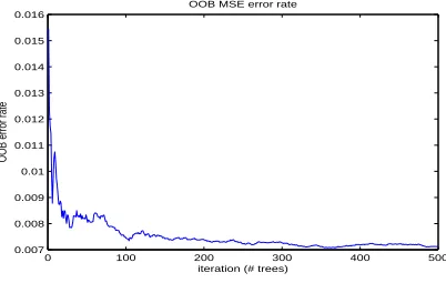
5.2.1 The Out-Of-Bag (OOB) Error Estimate
The training set for a tree is produced by testing with substitution. During this process, something like one-third of the cases are left out of the sample. These cases are considered as out-of-bag (OOB) data. It helps in getting an impartial evaluation of the regression error value as the forest develops. OOB data also helps in getting estimation of variable importance. In RF, as
the OOB is calculated internally during the run. Cross-validation of data or a different test set to obtain an im-partial evaluation of the test error is not required. The computation procedure for OOB is explained below.
• During construction of each tree, an alternate boot-strap sample from the original data is used. Some-thing like one-third of the cases from the bootstrap sample are left out and not used in the tree con-struction process.
• These OOB samples are put down thekth tree to obtain a regression. Using this process, a test set is acquired for each one case.
• At the end, supposej be the predicted value that is acquired by computing the average prediction value of forest, each time casenwas oob. The ex-tent of timesjis not equivalent to the actual value ofnaveraged over all cases is called as the out-of-bag error estimate.
The RF prediction accuracy can be determined from these OOB data by using the following formula.
OOB−M SE= 1
F
F
X
i=1
(yi−y¯iOOB)2 (4)
wherey¯iOOBrepresents the average prediction value of
ith observation from all trees for which this observation has been OOB.Fdenotes the no. of trees in the forest andyirepresents the actual value.
0 100 200 300 400 500
0.007 0.008 0.009 0.01 0.011 0.012 0.013 0.014 0.015 0.016
OOB MSE error rate
iteration (# trees)
OOB error rate
Figure 7:OOB MSE Error Rate
value. After some period, OOB error rate remains con-stant.
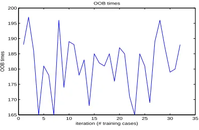
0 5 10 15 20 25 30 35
165 170 175 180 185 190 195 200
OOB times
iteration (# training cases)
OOB times
Figure 8:Number of Times Out Of Bag Occurs
Figure 8 displays the number of times, cases are out of bag for all training attributes. In this case, one hun-dred twenty number of training attributes are used.
5.2.2 Proximities
Proximity is one of the important data objects while cal-culating effort using RF technique. It measures the fre-quency of ending up the unique pairs of training sam-ples in the same terminal node. It also helps in filling up the missing data in the dataset and calculating number of outliers.
0 10
20 30
40
0 10 20 30 40
0 0.2 0.4 0.6 0.8 1
Training cases Training Cases
Proximity
Figure 9:Proximity
Figure 9 describes the proximity value generated using random forest technique. A 120 ×120 matrix used for generating the above figure. From the figure, it is observed that, for diagonal elements, the proximity value is maximum (equals to one). But for all other elements, the proximity value is less than one. The symmetric portion adjacent to diagonal area represents other elements proximity values.
Originally, a NxN matrix is formed by the proxim-ities. Once a tree is developed, all the data i.e.,
train-ing data and out-of-bag data are put down the tree. Its proximities should be increased by one, if it is found that two cases are in the same terminal node. Finally, the normalized values of the proximities are obtained by dividing with the number of trees.
5.2.3 Complexity
In the proposed approach, 500 number of trees are taken into consideration for implementing RF technique. In the usual tree growing algorithm, all descriptors are tested for their splitting performance at each node; while Random Forest only testsmtry of the descrip-tors. Sincemtry is typically very small, the search is very fast.
To get the right model complexity for optimal pre-diction strength, some pruning is usually done via cross validation for a single decision tree. This process can take up a significant portion of the computations. RF, on the other hand, does not perform any pruning at all. It is observed that in cases where there are an exces-sively large number of descriptors, RF can be trained in less time than a single decision tree. Hence, the RF algorithm can be very efficient.
5.2.4 Outlier
The cases that are expelled from the principle group of data and whose proximities to all different cases in the data mostly small are defined asOutliers. The concept of outliers can be revised by defining outliers relative to corresponding cases. In this way, an outlier is case whose proximities to all different cases are little. The average proximity is specified as:
¯
P(n) =
N
X
1
prox2(n, k) (5)
wherenandkdenote a training case in the regression andN represents the total no. of training cases in the forest. The raw outlier measure for casenis specified as:
nsample/P¯(n) (6) The result of raw outlier measure inversely depends on the average proximities. The average of these raw measures and their deviations from the average are as-certained for each one cases. The final outlier measure is obtained by subtracting the average from every raw measure, and afterwards dividing it by absolute devia-tion.
0 5 10 15 20 25 30 35 100
120 140 160 180 200 220 240 260 280
Training cases
Outlier
mean outlier outlier
Figure 10:Outlier
cases. The outlier value is dependent on the proxim-ity value generated using RF technique, which means that the outlier value is higher for lower proximity value and vice versa. Figure 10 displays the deviation of out-lier value from the mean outout-lier. The training cases for which the outlier value is higher, will generate the predicted effort value deviated more from actual effort value.
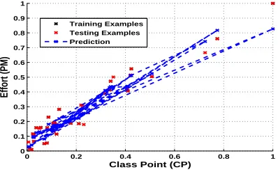
0 0.2 0.4 0.6 0.8 1
0 0.1 0.2 0.3 0.4 0.5 0.6 0.7 0.8 0.9 1
Class Point (CP)
Effort (PM)
Training Examples Testing Examples Prediction
Figure 11:Random Forest Technique-based Effort Estimation Model
0 0.2 0.4 0.6 0.8 1
0 0.1 0.2 0.3 0.4 0.5 0.6 0.7 0.8 0.9 1
Actual Effort (PM)
Predicted Effort (PM)
y=x Predicted Effort
Figure 12:Variation of Predicted Effort from Actual Obtained using
Random Forest Technique
This deviation is clearly visible from figure 11 and
12. Figure 11 and 12 displays the final effort estima-tion model obtained using RF technique. These figures show the variation of actual effort from the predicted result obtained using RF technique.
5.3 Performance Measures
The performance of the various models might be as-sessed by utilizing the accompanying criteria [13]:
• The Magnitude of Relative Error (MRE) is a very common criterion used to evaluate software cost estimation models. The MRE for each obser-vation i can be obtained as:
M REi =
|xi−yi|
¯
y (7)
where
xi= Actual Effort ofithtest data.
yi= Predicted Effort ofithtest data.
N = Total number of data in the test set.
• The Mean Magnitude of Relative Error (MMRE)can be achieved through the summation of MRE over N observations
M M RE=
N
X
1
M REi (8)
where
N = Total number of data in the test set.
• The Prediction Accuracy (PRED) is computed as:
P RED= (1−(
PN
i=1|xi−yi|
N ))∗100 (9)
where
N = Total number of data in the test set.
6 Comparison
The SGB algorithm and Decision Tree Forests algo-rithm exhibit functional similarity, because SGB cre-ates a tree ensemble, and also uses randomization dur-ing the creations of the trees. It creates a series of trees, and the prediction accuracy is calculated by feeding the result obtained from one tree to the next tree in the se-ries. However, RF builds trees in parallel and also uses voting method on the prediction.
Table 1: Comparison of Prediction Accuracy Values of Related Works
Sl.
No. Related Papers
Technique Used
Prediction Accuracy
1 Gennaro Costagliola et al. [5] Regression
Analysis 83%
2 Wei Zhou and Qiang Liu [25] Regression
Analysis 83%
3 S. Kanmani et al. [9] Neural
Network 87% 4 S. Kanmani et al. [10] Fuzzy Logic 92%
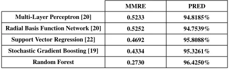
maximum of 92% prediction accuracy is achieved us-ing fuzzy logic technique. Finally, the results obtained in related work section is compared with results of pro-posed approaches, which is shown in table 2. The results obtained using proposed technique shows im-provement in the prediction accuracy value.
Table 2:Comparison of MMRE and PRED Values between the MLP,
RBFN, SVR, SGB and Random Forest Techniques
MMRE PRED
Multi-Layer Perceptron [20] 0.5233 94.8185%
Radial Basis Function Network [20] 0.5252 94.7539%
Support Vector Regression [22] 0.4692 95.8088%
Stochastic Gradient Boosting [19] 0.4334 95.3261%
Random Forest 0.2730 96.4250%
At the point when utilizing the MMRE, and PRED in assessment, good outcomes are entailed by lower es-timations of MMRE and higher eses-timations of PRED. Table 2 demonstrates the comparison of MMRE and PRED values for the MLP, RBFN, SVR, SGB and RF techniques. The MLP, RBFN, SVR and SGB tech-niques are already been applied over class point ap-proach with the help of same dataset as used while applying RF technique. This comparative study helps in accurately assessing the performance obtained using RF technique and proves that the results obtained us-ing RF technique-based effort estimation model outper-forms the results obtained using other existing models.
7 Conclusion
Several approaches have been considered by searchers and practitioners to calculate the effort re-quired to develop a given software product. However, the class point model is one of the effort estimation models which is used because of its simplicity, fastness and accurateness to a certain degree. In this paper, the proposed optimized class point model has been imple-mented using the RF technique and generated results are compared with the results obtained from the MLP,
RBFN, SVR and SGB techniques. The results demon-strate that the random forest technique provides lower estimates of MMRE and higher estimates of prediction accuracy. Consequently, it could be inferred that effort estimation utilizing the random forest technique outper-forms other machine learning techniques. The compu-tations for above procedure were implemented, and the outputs were generated using MATLAB. Extension to this procedure might be made by applying other ma-chine learning techniques on the class point approach.
References
[1] Baskeles, B., Turhan, B., and Bener, A. Software effort estimation using machine learning methods. InComputer and information sciences, 2007. iscis 2007. 22nd international symposium on, pages 1– 6. IEEE, 2007.
[2] Breiman, L. Random forests. Machine learning, 45(1):5–32, 2001.
[3] Carbone, M. and Santucci, G. Fast&&serious: a uml based metric for effort estimation. In Proceedings of the 6th ECOOP Workshop on Quantitative Approaches in Object-Oriented Soft-ware Engineering (QAOOSE’02), pages 313–322, 2002.
[4] Costagliola, G., Ferrucci, F., Tortora, G., and Vi-tiello, G. Towards a software size metrics for object-oriented systems. Proc. AQUIS, 98:121– 126, 1998.
[5] Costagliola, G., Ferrucci, F., Tortora, G., and Vi-tiello, G. Class point: an approach for the size estimation of object-oriented systems. Software Engineering, IEEE Transactions on, 31(1):52–74, 2005.
[6] Elish, M. O. Improved estimation of soft-ware project effort using multiple additive regres-sion trees. Expert Systems with Applications, 36(7):10774–10778, 2009.
[7] Elyassami, S. and Idri, A. Evaluating software cost estimation models using fuzzy decision trees. Recent Advances in Knowledge Engineering and Systems Science, WSEAS Press, pages 243–248, 2013.
[9] Kanmani, S., Kathiravan, J., Kumar, S. S., and Shanmugam, M. Neural network based effort es-timation using class points for oo systems. In Pro-ceedings of the International Conference on Com-puting: Theory and Applications, ICCTA ’07, pages 261–266, Washington, DC, USA, 2007. IEEE Computer Society.
[10] Kanmani, S., Kathiravan, J., Kumar, S. S., and Shanmugam, M. Class point based effort estima-tion of oo systems using fuzzy subtractive cluster-ing and artificial neural networks. InProceedings of the 1st India software engineering conference, ISEC ’08, pages 141–142, New York, NY, USA, 2008. ACM.
[11] Kim, S., Lively, W., and Simmons, D. An effort estimation by uml points in early stage of soft-ware development. Proceedings of the Interna-tional Conference on Software Engineering Re-search and Practice, pages 415–421, 2006. [12] Matson, J., Barrett, B., and Mellichamp, J.
Soft-ware development cost estimation using function points. Software Engineering, IEEE Transactions on, 20(4):275–287, 1994.
[13] Menzies, T., Chen, Z., Hihn, J., and Lum, K. Selecting best practices for effort estima-tion. Software Engineering, IEEE Transactions on, 32(11):883–895, 2006.
[14] Nassif, A. B. Enhancing use case points esti-mation method using soft computing techniques. Journal of Global Research in Computer Science, 1(4):12–21, 2010.
[15] Nassif, A. B., Capretz, L. F., and Ho, D. Es-timating software effort based on use case point model using sugeno fuzzy inference system. In Tools with Artificial Intelligence (ICTAI), 2011 23rd IEEE International Conference on, pages 393–398. IEEE, 2011.
[16] Nassif, A. B., Capretz, L. F., and Ho, D. Estimat-ing software effort usEstimat-ing an ann model based on use case points. InMachine Learning and Appli-cations (ICMLA), 2012 11th International Confer-ence on, volume 2, pages 42–47. IEEE, 2012. [17] Nassif, A. B., Ho, D., and Capretz, L. F.
Regres-sion model for software effort estimation based on
the use case point method. In2011 International Conference on Computer and Software Modeling, volume 14, pages 106–110. IACSIT Press, Singa-pore, 2011.
[18] Pahariya, J., Ravi, V., and Carr, M. Software cost estimation using computational intelligence tech-niques. InNature & Biologically Inspired Com-puting, 2009. NaBIC 2009. World Congress on, pages 849–854. IEEE, 2009.
[19] Satapathy, S. M., Acharya, B. P., and Rath, S. K. Class point approach for software effort esti-mation using stochastic gradient boosting tech-nique. SIGSOFT Softw. Eng. Notes, 39(3):1–6, June 2014.
[20] Satapathy, S. M., Kumar, M., and Rath, S. K. Class point approach for software effort estima-tion using soft computing techniques. In Ad-vances in Computing, Communications and Infor-matics (ICACCI), 2013 International Conference on, pages 178–183. IEEE, 2013.
[21] Satapathy, S. M., Kumar, M., and Rath, S. K. Fuzzy-class point approach for software effort es-timation using various adaptive regression meth-ods. CSI Transactions on ICT, 1(4):367–380, 2013.
[22] Satapathy, S. M. and Rath, S. K. Class point ap-proach for software effort estimation using vari-ous support vector regression kernel methods. In Proceedings of the 7th India Software Engineer-ing Conference, ISEC ’14, pages 4:1–4:10, New York, NY, USA, 2014. ACM.
[23] Sheta, A. Software effort estimation and stock market prediction using takagi-sugeno fuzzy mod-els. In Fuzzy Systems, 2006 IEEE International Conference on, pages 171–178. IEEE, 2006.
[24] Sivanandam, S., Sumathi, S., Deepa, S., et al. Introduction to fuzzy logic using MATLAB, vol-ume 1. Springer, 2007.