Vol. 2 Issue 7, July - 2016
Optimal Planning of Distribution Generation for
Distribution Network Regarding to Losses
Energy and Harmonic Reduction
Sepideh Rajabi1 , HeidarAli Shayanfar2 and Faramarz Faghihi3
Abstract—Simultaneous use of nonlinear loads
and renewable distributed generation resources with improper allocation in the distribution network creates harmonic distortions and the electrical energy losses. In order to control harmonic distortions and reduce energy losses
can be optimized planning with various
combinations of renewable sources prepared. To prove the effectiveness of the proposed method, a
31-buses distributions network including
renewable and non-renewable distributed
generation resources, non-linear loads and Shunt capacitors can be employed using genetic algorithm. In addition to harmonic load flow based on forward/backward sweep via MATLAB software is analyzed.
Keywords—Genetic Algorithm, Non-Linear Loads, Distribution Generation and Harmonic Distortions
1. Introduction
Due to the increasing demand for high quality electric energy consumption and limitations on fossil fuels, the use of renewable energy resources in distribution systems has increased. Distributed generation resources in distribution networks are used to reduce the power losses in the power plants and distribution and transmission networks and to improve power quality and network reliability. Improper placement of distributed generationunits will not only increase the losses but also causes system performance problems [1].
In addition, due to increasing non-linear loads in distribution networks, the optimal allocation of distributed generation resources in the presence of capacitors and non-linear loads is so crucial. Non-linear loads and renewable energy resources cause harmonic distortions because of using converters.
1,3. Islamic Azad University, Science and Research Branch, Faculty of Electrical and Computer, Electrical Engineering Group,Tehran-Iran,[email protected],2. [email protected] 2.Center of Excellence for Power System Automation and Operation, School of Electrical Engineering, Iran
University of Science and Technology, Tehran- Iran,[email protected]
Thus optimal planning for the proposed system must be noticed [2,3].
Artificial algorithms can be used for optimal planning of the distribution system components, including capacitors and distributed generationresources. For example, the artificial algorithm bee colony is used to determine the optimal sizing of distributed generation in order to optimize the active power [4,5]. In order to have losses reduction and voltage profile improvement considering stability and capacity of distribution lines in a 33-buses and 69-buses network, genetic algorithms have been used for optimal capacitor placement and distributed generation resources [6]. [7,8] the optimal capacitor placement in radial distribution system is done to reduce losses and to improve voltage profile considering economic dispatch using fuzzy systems.
In this paper, in order to achieve the optimal allocation of distributed generation resources with several scenarios in the presence of non-linear loads and shunt capacitors for the network including harmonic distortions, the harmonic load flow method using forward/backward sweep is used and genetic algorithms have also been used for the optimal placement of distributed generation resources for reducing energy losses. The objective function includes the annual energy losses and voltage restrictions on different buses, total harmonic distortions and penetration limits and candidate buses for the installation of distributed generationresources. The proposed method is applied on a 31-buses system and the simulation results in MATLAB software show the ability of the proposed method to improve the energy losses and total harmonic distortions [9,10,2].
2. Background
Vol. 2 Issue 7, July - 2016 generation and the power quality are studied and then
a definition for the harmonic load flow and genetic algorithm for optimal planning is presented [2].
2-1 Distributed Generation
The comprehensive and unrestricted definition of distributed generation resources is as follows : The electrical energy source which is directly connected to the distribution network or consumer and supplies a part of the network power consumption [11,12,13]. In this paper wind turbines and solar cells as well as a non-renewable source are used.
2-2 Power Quality
The power quality includes the specifications of the power network which provide the ability to function adequately for the equipment. Regarding the power quality, the consumers' opinions are in priority. Any changes in the quantities of voltage, current, and frequency causing the failure or improper performance of consumers' equipment affect the power quality. Harmonics are one of the important factors reducing the power quality [14,15].
2-3 Load Flow
Designing and exploiting a power system aims to supply the loads required for the network. Load flow computes the electrical quantities of a power system in a steady-state for determined and specific loads [16,17,18]. In this paper, forward/backward sweep is the method of load flow.
2-4 Genetic Algorithms
Genetic algorithm is a statistical method for optimization and search. The basic idea of this approach is driven from the Darwinian evolutionary theory. This algorithm is used for optimal placement of distributed generation in order to reduce annual energy losses [19].
3. Problem and Modeling 3.1 Statement of the problem
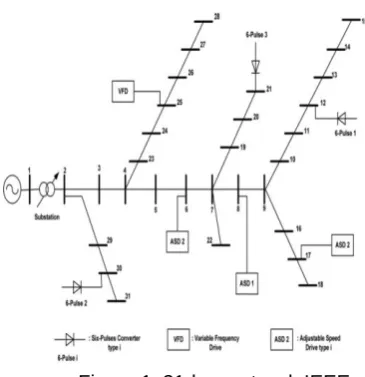
A 31-buses distribution network IEEE is investigated. This network consists of seven non-linear loads and 3 types of distributed generation resources and 7 shunt capacitors. Renewable distributed generation resources include wind turbines and solar cells and there also is a non-renewable distributed generation resource with a fixed power. To minimize annual energy losses and harmonic control, genetic algorithm and load flow technique with the use of forward/backward sweep method in the MATLAB software are used [2].
Figure 1. 31-bus network IEEE
3.1.1 Objective Function
Objective function is the optimal allocation of distributed generation resources to reduce annual energy losses:
OF=Min{Plossyear} (1)
Assumptions considered in this regard include the following items:
A. Only one type of distributed generation resource can be connected to a bus.
B. All units of distributed generation are able to work in unity power factor.
C. A local distribution company should not make any improvement in the system.
Distribution system studied assumed on the maximum limit for investment in capacity on any bus and to determine the optimal mix of distributed energy resourses of 5 scenarios considered
2
(h) (h) (h) 2
1
.
[R]
.[I ]
nb
T
Loss ij i ij
i
P
B
R
A
(2)Where nb is the number of branches and R is the matrix of line resistance and h is the number of harmonics.
3.1.2 Limitations
Provisions intended for this problem include [2,3]:
- The size and angle of the slack bus voltage:
1
1,
10.0
V
(3)- Voltage limitation in buses:
min BUS max
V
V
V
(4)- Line capacity constraints: max
Vol. 2 Issue 7, July - 2016
- THD constraints:
max
BUS
THD
THD
(6)- Limitations on the number of buses:
n =6-8-12-13-15-17-18-20-21-25-28-30-31
3-2 Harmonic Load Flow Method
Due to non-linear loads and renewable distributed generation resources, harmonic analysis of the distribution network is of importance. The analysis determines the amount of harmonic distortions in different buses of the distribution network and the way they can be removed. Forward/backward sweep is a powerful technique that is used in the distribution system. However, because of frequencies similar to capacitors' resonance frequency, this method cannot be directly used until the harmonic currents absorbed by the bus capacitors of distributed networks are not determined. After determining the currents absorbed by the capacitors, this method can be used to find out the relationship between bus harmonic currents, line currents, and harmonic rank of bus voltages [20,21,22].
3-2-1 Current Backward Sweep
Current harmonics can be described by the following vector:
(7)
Ih and Is are the harmonic flows injected by non-linear
loads and linear impedances absorbed by the shunt capacitors in the h harmonic order, respectively. For distribution systems with m harmonic resources and n shunt capacitors, the current vector rank will be (m + n) × 1. Then, a coefficient vector will be defined, which describes the current flow among the branches:
( 8 ) (h ),k ij (h ),k ij (h ),k ij
Ah
A
As
( 9 ) T (h),k (h ),k (h),kij ij
B
A
I
Here, the coefficient vector of harmonic currents between i and j buses is in the h-order harmonic and they are vectors of harmonic current coefficients injected by non-linear loads and linear impedance and harmonic currents absorbed by the shunt capacitors between i and j buses in the h-order harmonic.
Line voltage drop caused by the system harmonic vector will be as follows:
(10)
[HA (h)] is the connecting matrix between the bus
voltage vector and the system harmonic vector and [Has (h)] is composed of row vectors in accordance
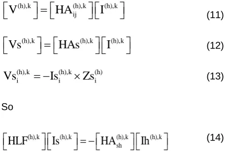
with the buses of the shunt capacitors. This relationship can be written as follows:
(11) (h),k (h),k (h),k
ij
V
HA
I
(12) (h),k (h),k (h),k
Vs
HAs
I
(13) (h),k (h),k (h)
i i i
Vs
Is
Zs
So
(14) (h),k (h),k (h),k (h),k
sh
HLF
Is
HA
Ih
3-2-2Current Forward Sweep
Now, one can easily calculate line current, voltage drop and the voltage of buses caused by harmonic currents:
(h),k 1 (h),0 (h),k
V
V
V
(15)Now, this repetition for h-order harmonic continues until the following criterion is reached:
(16) (h),k 1 (h),k
i i
V
V
for i 1
N
3.3 Modeling Components 3-3-1 Load Model
Load model is generated by using the IEEE-RTS system in which the data on the intensity of solar radiation and wind speed are modeled hourly by beta and weibull Pdfs. Each year is divided into four
seasons and one day is considered to represent that season. Therefore, there will be 96 different time sections
Vol. 2 Issue 7, July - 2016
Figure 2. Load Model
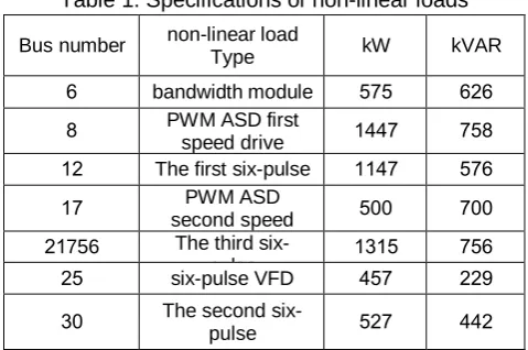
Table 1. Specifications of non-linear loads
Bus number non-linear load
Type kW kVAR 6 bandwidth module 575 626
8 PWM ASD first
speed drive 1447 758 12 The first six-pulse 1147 576
17 PWM ASD second speed
drive
500 700
756
21 The third six-pulse
1315 756 25 six-pulseVFD 457 229
30 The second
six-pulse 527 442
3-3-2 Wind Speed Model
A common expression for the wind speed is a function of rail probability density [12]:
(17 )
2 2
2
(v)
v
exp( (v/ c) )
f
c
(18 ) 2
2
0 0 2
2
( )
exp( ( / ) ) dv
/ 2
m
v
v
vf v dv
v c
c
1.128
mc
V
Where v is the wind speed and c is the scale parameter.
Figure 3. Annual curve of the wind speed in the studied problem
3-3-3 Intensity of the Solar Radiation Model
Beta probability density function is used for the intensity of solar radiation.
( 1) ( 1)
(
)
(1
)
( ) ( )
( )
,0 s 1
0,
bs
s
f s
ow
(19)Where s is the intensity of solar radiation in
kW
/
m
2 , f probability density function. S,
and
are parameters of unction Γ. Figure 3 and 4 show the annual curve of wind speed and the annual curve of the solar radiation in the studied system, respectively.Figure 4. Annual solar radiation intensity curve
3-4 Calculating Output Power 3.4.1 Wind Turbine
Based on the available information on the wind turbine, the output power is calculated based on the following equation:
(20)
The output power of a wind turbine depends on the wind speed.
3-4-2 Solar Cell
Vol. 2 Issue 7, July - 2016
3-5 Scenario Plans
Scenario 1: In this scenario, none of the distributed generation resources is not connected to the system. Scenario 2: In this case, only non-renewable distributed generation resource with fixed power is connected to the distribution network.
Scenario 3: In this scenario, a single wind turbine and the non-renewable distributed generation resource are added to the system.
Scenario 4: There are a solar unit and a non-renewable distributed generation resource in the system.
Scenario 5: In this scenario, two wind turbines and a solar unit are added to the system.
4-Simulation and Comparison of the Selected Scenarios
4.1 Scenario 1
In this scenario in which none of the distributed generation resources is not connected to the system, the annual energy loss is equal to1:
Ploss=
1.4964 10
7kWh
Figure 5. The curve of annual losses in watts for the scenario 1
Figure 6. The maximum THD on an annual basis for the scenario 1
1 In order to optimize, GA tool of the MATLAB
software is used.
4.2 Scenario 2:
In this case, a single non-renewable distributed generation unit as much as 6.5 MW at bus No. 6 is the optimal result of this scenario and the losses in this case are equal to:
7
1.2346 10
kWh
=
loss
P
Figure 7. Annual losses curve resulting from Scenario 2
Figure 8. The maximum THD on an annual basis for the scenario 2
Vol. 2 Issue 7, July - 2016
4.3 Scenario 3:
The non-renewable unit with 15% of contribution and the wind unit with 85% of contribution are connected to the bus No. 30 and the bus No. 17, respectively. In this case, the annual losses will be equal to
7
1.1757 10
kWh
.Figure 10. The annual losses curve resulting from Scenario 3
Figure 11. The maximum THD on an annual basis for the scenario 3
Figure 12. The objective function curve obtained from the genetic algorithm for scenario 3
4.4 Scenario 4:
In this scenario, the non-renewable unit with 10% of contribution and the solar unit with 90% of contribution are connected to the bus No. 18 and the bus No. 28, respectively. In this case, the annual losses will be
equal to Ploss=
7
1.1757 10
kWh
.Figure 13. The annual losses curve resulting from Scenario 4
Figure 14. The maximum THD on an annual basis for the scenario 4
Vol. 2 Issue 7, July - 2016
4.5 Scenario 5:
In this case, a wind unit with 15% of contribution and a wind unit with 90% of contribution are connected to the bus No. 6 and the bus No. 25, respectively. Moreover, a solar unit with 52% of contribution is connected to the bus No.17. In this case, the annual losses will be equal to:
Ploss=
1.1763 10
7kWh
Figure 16. The annual losses curve resulting from Scenario 5
Figure 17. The maximum THD on an annual basis for the scenario 5
Figure 18. The objective function curve obtained from the genetic algorithm for scenario 5
4-6 Results of Solar and Wind Resources
Placement Based on Genetic Algorithm Analysis
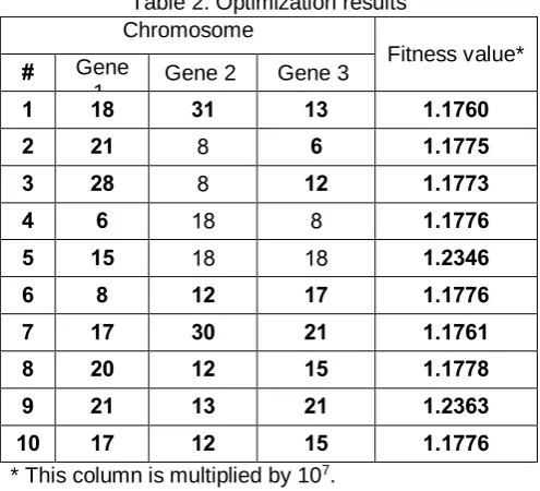
To address the issue, a genetic algorithm which produces 10 chromosomes per iteration is used. Each chromosome shows the position of distributed generation resources and their genes represent the position of each resource. The first and second genes show the position of the first and second wind turbines, respectively. The third gene shows the position of solar power plant in the micro-grid. This table shows the investigation results of a generation:
Table 2. Optimization results Chromosome
Fitness value*
# Gene
1 Gene 2 Gene 3
1 18 31 13 1.1760
2 21 8 6 1.1775
3 28 8 12 1.1773
4 6 18 8 1.1776
5 15 18 18 1.2346
6 8 12 17 1.1776
7 17 30 21 1.1761
8 20 12 15 1.1778
9 21 13 21 1.2363
10 17 12 15 1.1776
* This column is multiplied by 107.
4.7 Analysis Based on Losses in Scenarios 1 and 5 in Summer:
Vol. 2 Issue 7, July - 2016 Table 3. Comparison of Scenarios 1 and 5 regarding
the losses
Hour Scenario 1
Scenario 5
Percentage of drop
1 11.8825 10.2650 13.6162
2 10.5061 9.0759 13.6162
3 9.5293 8.2321 13.6162
4 9.2143 7.9600 13.6162
5 9.2143 7.9600 13.6162
6 9.5293 8.2321 13.6153
7 14.4957 12.5224 13.6107
8 19.5794 16.9141 13.6012
9 23.8931 20.6406 13.5917
10 24.4001 21.0785 13.5781 11 24.4009 21.0792 13.5703 12 23.8957 20.6428 13.5654 13 23.8954 20.6426 13.5572 14 23.8949 20.6421 13.5408 15 22.8982 19.7811 13.5530 16 23.3916 20.2073 13.5822 17 25.9444 22.4126 13.6019 18 26.4704 22.8670 13.6084 19 26.4703 22.8669 13.6159 20 24.3951 21.0742 13.6157 21 21.9201 18.9361 13.6162 22 18.2354 15.7530 13.6162 23 14.1060 12.1858 13.6162
24 10.5061 9.0759 13.6162
Figure 19. Comparison of scenarios 1 and 5 based on losses (lower: Scenario 5 and upper: Scenario 1)
4-8 Analysis Based on Maximum Harmonic Distortion
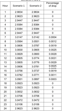
Reviewing the maximum THE in the scenarios 1 and 2 in the summer in Table 4 shows that using a non- renewable distributed generation resource reduces THD.
Table 4. The results of maximum THD in the scenarios 1 and 2
Hour Scenario 1 Scenario 2
Percentage of drop
1 2.9834 2.9834 0
2 2.9623 2.9623 0
3 2.9447 2.9447 0
4 2.9384 2.9384 0
5 2.9384 2.9384 0
6 2.9447 2.9447 0
7 3.0147 3.0142 0.0004
8 3.0564 3.0551 0.0012
9 3.0806 3.0787 0.0019
10 3.0830 3.0805 0.0025
11 3.0829 3.0800 0.0029
12 3.0805 3.0774 0.0031
13 3.0805 3.0776 0.0029
14 3.0806 3.0781 0.0025
0.0025 0.0025
15 3.0756 3.0737 0.0019
16 3.0782 3.0771 0.0011
17 3.0901 3.0897 0.0003
18 3.0923 3.0923 0
19 3.0923 3.0923 0
20 3.0832 3.0832 0
21 3.0706 3.0706 0
22 3.0472 3.0472 0
23 3.0106 3.0106 0
24 2.9623 2.9623 0
Vol. 2 Issue 7, July - 2016 Table5- THD maximum between the two scenarios 1
and 2b
Hour Scenario 1 Scenario 2b
Percentage of drop
1 2.9834 2.7033 9.3885
2 2.9623 2.6721 9.7957
3 2.9447 2.6466 10.1220
4 2.9384 2.6377 10.2349
5 2.9384 2.6377 10.2349
6 2.9447 2.6466 10.1220
7 3.0147 2.7507 8.7552
8 3.0564 2.8166 7.8431
9 3.0806 2.8564 7.2765
10 3.0830 2.8600 7.2320
11 3.0829 2.8597 7.2426
12 3.0805 2.8554 7.3076
13 3.0805 2.8556 7.3028
14 3.0806 2.8559 7.2919
15 3.0756 2.8480 7.3993
16 3.0782 2.8529 7.3185
17 3.0901 2.8736 7.0052
18 3.0923 2.8777 6.9404
19 3.0923 2.8777 6.9405
20 3.0832 2.8621 7.1702
21 3.0706 2.8409 7.4788
22 3.0472 2.8025 8.0285
23 3.0106 2.7447 8.8319
24 2.9623 2.6721 9.7957
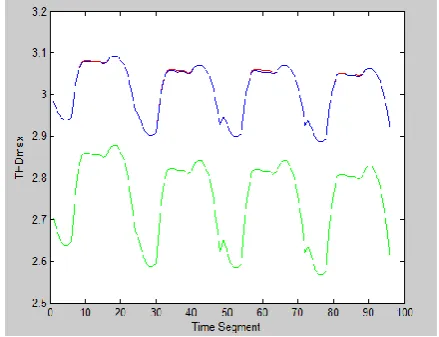
Light diagram is related to the new scenario and shows lower THD compared to the dark diagram.
Figure 20. Comparative diagrams of the annual maximum THD figures for scenarios 1, 2 and 2 B
(respectively upper, top of the upper and lower)
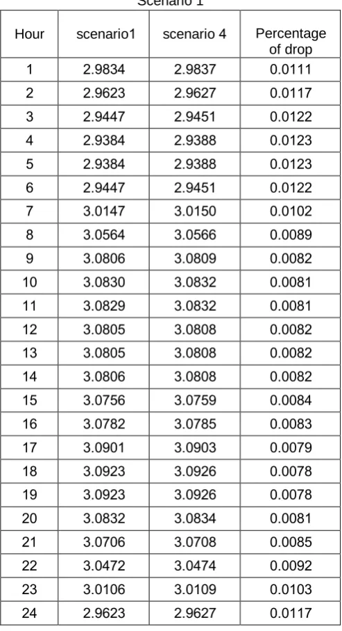
4-9 Analysis Based on Maximum Harmonic Distortion Generation in The Scenarios 1 and 4
In scenario 1, only non-linear loads act as a resource of harmonic generation and in scenario 4, a solar source as a new harmonic source is added to this resources.
Figure 27 and Table 6 compares scenarios 1 and 4 of THDmax to show that.
Figure 21. Comparison of Scenarios 1 and 4 regarding THDmax (lower: Scenario 4 and upper:
Vol. 2 Issue 7, July - 2016 Table 6. THD increase for scenario 4 compared to
Scenario 1
Hour scenario1 scenario 4 Percentage of drop
1 2.9834 2.9837 0.0111
2 2.9623 2.9627 0.0117
3 2.9447 2.9451 0.0122
4 2.9384 2.9388 0.0123
5 2.9384 2.9388 0.0123
6 2.9447 2.9451 0.0122
7 3.0147 3.0150 0.0102
8 3.0564 3.0566 0.0089
9 3.0806 3.0809 0.0082
10 3.0830 3.0832 0.0081
11 3.0829 3.0832 0.0081
12 3.0805 3.0808 0.0082
13 3.0805 3.0808 0.0082
14 3.0806 3.0808 0.0082
15 3.0756 3.0759 0.0084
16 3.0782 3.0785 0.0083
17 3.0901 3.0903 0.0079
18 3.0923 3.0926 0.0078
19 3.0923 3.0926 0.0078
20 3.0832 3.0834 0.0081
21 3.0706 3.0708 0.0085
22 3.0472 3.0474 0.0092
23 3.0106 3.0109 0.0103
24 2.9623 2.9627 0.0117
According to the table, by adding a solar source as a new harmonic source to the THD system, the maximum for buses had a natural increase. However, due to low capacity injection into the manufacturers in this issue, this difference does not seem to be significant.
Figure 27 and Table 6 show the comparisons of Scenarios 1 and 4 in terms of THDmax.
Figure 21. Comparison of Scenarios 1 and 4 in terms of THDmax
Table 6. THD increase for Scenario 4 with respect to Scenario 1
5. Conclusion
In this paper, distributed generations were used to reduce losses in the harmonic polluted distribution system. This approach faces some critical challenges, one of which is the load flow in the distribution system despite the presence of harmonic loads. The
forward/backward sweep method was used to solve the problem. Another challenge is the issue of uncertainties in wind speed and solar radiation for the renewable distributed generations. For the purpose of resolving this issue, the railway and beta probability density functions are used. The use of renewable resources that are properly located significantly reduces the loss rate while they could have a negligible impact on THD which does not make it over the limit.
References
[1] Mostafa F.shaaban, Yasser M. Atwa, “DG Allocation for benfit maximization in distribution networks” IEEE Transaction on Power system, Vol. 28, No. 2, May 2013.
[2] Abdelazeem A.Abdelsalam, Ehab F. El-Saadany, “Probabilistic approach for optimal planning of distributed generators with controlling harmonic distortion” IET Generation, Transmission & Distribution, May 2013
[3] V.Ravikumar Pandi, H.H. Zeineldin, “Determining optimal location and size of distributed generation resources considering harmonic and protection coordination limits” IEEE Transaction on Power system, Vol. 28, No. 2, May 2013.
[4] Seyed Ali Arefifar, Yaser Abdel- Rady, “Probabilistic optimal reactive power planning in distribution systems with renewable resources in grid-connected and island modes” IEEE Transaction on Industrial Electronics, Vol. 47, No. 11, March 2013. [5] Abu-Mouti F.S, El- Hawary, “Optimal distributed grneration allocation and sizing in distribution system via artificial bee colony algorithm” IEEE Transaction on Power Delivery, Vol. 26, No. 2, May 2011, pp. 2090-2101.
[6] Moradi M.H., A. Zeinalzadeh, Y. Mohammady, “An effeicent hybrid method for solving the optimal sitting and sizing problem of DG and shunt capacitor banks simultaneously based on imperialist competitive algorithm and genetic algorithm” Electrical Power and Energy System, vol.54, 2014, pp. 101-11.
[7] Kannans S.M., Renuga P., Kalyani S. "Optimal capacitor placement and sizing using Fuzzy-DE and Fuzzy-MAPSO methods” Applied Soft Computing, Vol, 11, 2011, pp. 4997-5005.
[8] Sajjadi.S.M, Haghifaam M.R., Salehi J., “Simultaneous placement of distributed generation and capacitors in distribution network considering voltage stability index” International Journal of Electrical Power & Energy Systems, Vol. 46, 2013, pp. 366-375.
Vol. 2 Issue 7, July - 2016 [10] Vasileios A., Evangelopoulos S., Georgiakis,
“Evangelopoulos , Optimal distributed generation placement under uncertainties based on point estimate method embedded genetic algorithm” IET Generation, Transmission & Distribution, Vol. 8, 2014, pp. 389-400.
[11] McGowan,J.G., Manwell J.F., “Hybrid Wind/PV/Diesel system experiences” Renewable Energy, Vol. 16, No. 1-4, 1999, pp. 928-933.
[12] Ijumba N.M., Jimoh A.A., Nkabinde M., “Influence of distributed generation on distribution network performance” IEEE AFRICOW, Vol. 2, No. 28, 1999, pp. 961-964.
[13] Ackermann.T., Anderson G., “Distributed generation a definition” Elsevier Science, 2000. [14] Wagner V.E, Balda J.C., Griffith D.C., Mceachern A., Barnes T.M., Hartman D.P., Phileggi D.J., Emannuel A.E., Horton W.F., Reid W.E., “Effects of the harmonics on Equipments” IEEE Transaction on Power Delivery, Vol. 8, No. 2, 1994, pp. 672-680. [15] Antonio Bracale, Pierluigi Caramia, Guido carpinelli, “Site and system indices for power-quality characterization of distribution networks with distributed generation” IEEE Transaction on Power Delivery, Vol. 26, No. 3, July 2011.
[16] Shirmohammadi D., Hong H.W., Semlyn A., “A compensation – based power flow method for weakly meshed distribution and transmission networks” IEEE Transaction on Power Delivery, Vol. 3, No. 2, 1998, pp. 753-762.
[17] Cheng C.S., Shirmohammadi D., “A three-phase power flow method for real-time distribution system analysis” IEEE Transaction on Power system, Vol. 10, No. 2, 1995, pp. 671-679.
[18] Schlabbach J., Rpfalskik H. “Power system engineering planning, design and operation of power systems and equipment” Wiley, USA, 2000.
[19] Seyed Mahdi Mazaheri, Hassan Monsef, Ruben Romero, “A hybrid heuristic and evolutionary algorithm for distribution substation planning” IEEE Systems Journal, vol. 9, no. 4 Dec. 2015, pp. 1396-1408. [20] Teng J.H., hang Ch. Y. “A Fast harmonic load flow method for industrial distribution systems” International Conference on Power System Technology- China, 2000, pp. 1149-1154.
[21] Wanxing sheng, Ke-Yan Liu, Sheng Kemg, “Optimal power flow algorithm and analysis in distribution system considering distributed generation” IET Transmission & Distribution, Vol. 8, 2014, pp. 261-272 .