Forecasting Model For Enrolment Combining Weighted Fuzzy Time Series And Fourier Series Transform

(1)

Vol. 3 Issue 1, January - 2017

Forecasting Model for Enrolment Combining

Weighted Fuzzy Time Series and Fourier

Series Transform

Nghiem Van Tinh

Thai Nguyen University of Technology - Thai Nguyen University, Thai Nguyen, Vietnam

Nguyen Tien Duy

Thai Nguyen University of Technology - Thai Nguyen University, Thai Nguyen, Vietnam

Abstract—Fuzzy time series (FTS) methods was

first introduced by Song and Chissom (1993, 1994) based on the fuzzy set theory proposed by Zadeh (1965). Over the earlier few years, some methods have been presented based on fuzzy time series to forecast real problems, such as forecasting stock market, temperature prediction, forecasting enrolments, disease diagnosing, etc. Traditionally, time series forecasting problems are being solved using a class of Autoregressive moving average models. Being linear statistical models, they cannot build relationship among the nonlinear variables. Calculating the parameters for multi-variables is another issue faced by them. The strong relationship among these variables may result in large errors. Furthermore, a model cannot be estimated correctly if the historical data is less. Therefore, this paper, we propose a new fuzzy forecasting model to overcome the drawbacks of the traditional forecasting models that aim increasing the forecasting accuracy. In our studies, a hybrid forecasting model based on aggregated FTS and Fourier series analysis. Firstly, we propose weighted models to tackle two issues in fuzzy time series forecasting, namely, recurrence and weighting. Then, the using Fourier series to modify the residuals of the weighted FTS for improving the forecasting performance. By using the enrolment data at the University of Alabama from 1971s to 1992s as the forecasting target, the empirical results show that the proposed model outperforms one of the conventional FTS models

Keywords — Fuzzy time series(FTS), fuzzy logical relationship groups (FLRG), forecasting,

Fourier series, enrollments.

I. INTRODUCTION

Fuzzy time series procedures, which have attracted the attention of many researchers in recent years, have a quite wide area of use, such as information technology, economy, environmental sciences and hydrology and it play an important role in our daily life. Therefore, many more forecasting models have been developed to deal with various problems in order to help people to make decisions, such as crop forecast [6], [7] academic enrolments [1], [10], the temperature prediction [13], stock markets [14], etc. There is the matter of fact that the traditional forecasting methods cannot deal with the forecasting problems in which the

historical data are represented by linguistic values. Ref. [1], [2] proposed the time-invariant FTS and the time-variant FTS model which use the max–min operations to forecast the enrolments of the University of Alabama. However, the main drawback of these methods is enormous computation load. Then, Ref. [3] proposed the first-order FTS model by introducing a more efficient arithmetic method. After that, FTS has been widely studied to improve the accuracy of forecasting in many applications. Ref. [4] considered the trend of the enrolment in the past years and presented another forecasting model based on the first-order FTS. He pointed out that the effective length of the intervals in the universe of discourse can affect the forecasting accuracy rate. In other words, the choice of the length of intervals can improve the forecasting results. Ref. [5] presented a heuristic model for fuzzy forecasting by integrating Chen’s fuzzy forecasting method [3]. At the same time, Ref.[8] proposed several forecast models based on the high-order fuzzy time series to deal with the enrolments forecasting problem. In [9], the length of intervals for the FTS model was adjusted to forecast the Taiwan Stock Exchange (TAIEX).

Clearly, fuzzy time series model has been applied to environmental sciences, business and engineering; however, fuzzy time series model is still necessary to overcome its drawbacks. In order to cope with these drawbacks in the fuzzy time series model, residual analysis becomes quite important in order to reuse some possible useful information [19].

In this paper, we proposed a hybrid forecasting model combining the weighted fuzzy relationship groups and Fourier series technique. In case study, we applied the proposed method to forecast the enrolments of the University of Alabama. Computational results show that the proposed model outperforms other existing methods.

The rest of this paper is organized as follows. A brief review of the theory of fuzzy time series is described in Section 2. In Section 3, a novel forecasting model base on the weighted fuzzy time series and Fourier series transform. Experiments are presented in Section 4, and some concluding remarks are given in Section 5.

II. FUZZY TIME SERIES

In this section, we provide briefly some definitions of fuzzy time series.

In [1], [2] Song and Chissom proposed the definition of fuzzy time series based on fuzzy sets, Let

(2)

Vol. 3 Issue 1, January - 2017 is defined as A={ fA(u1)/u1+…+fA(un)/un }, where fA is a

membership function of a given set A, fA :U [0,1], fA(ui) indicates the grade of membership of ui in the

fuzzy set A, fA(ui) ϵ [0, 1], and 1≤ i ≤ n . General

definitions of fuzzy time series are given as follows:

Definition 1: Fuzzy time series

Let Y(t) (t = ..., 0, 1, 2 …), a subset of R, be the

universe of discourse on which fuzzy sets fi(t) (i = 1,2…) are defined and if F(t) be a collection of fi(t)) (i = 1, 2…). Then, F(t) is called a fuzzy time series on Y(t)

(t . . ., 0, 1,2, . . .).

Definition 2: Fuzzy logic relationship

If there exists a fuzzy relationship R(t-1,t), such that F(t) = F(t-1) R(t-1,t), where " " is an max - min arithmetic operator, then F(t) is said to be caused by F(t-1). The relationship between F(t) and F(t-1) can be denoted by F(t-1)→ F(t). Let Ai = F(t) and Aj = F(t-1), the relationship between F(t) and F(t -1) is denoted by fuzzy logical relationship Ai → Aj where Ai and Aj refer to the current state or the left hand side and the next state or the right-hand side of fuzzy time series.

Definition 3: 𝜆- order fuzzy time series

Let F(t) be a fuzzy time series. If F(t) is caused by F(t-1), F(t-2),…, F(t-𝜆+1) F(t-𝜆) then this fuzzy relationship is represented by by F(t-𝜆), …, F(t-2), F(t-1)→ F(t) and is called an 𝝀- order fuzzy time series.

Definition 4: Fuzzy Relationship Group (FLRG) Fuzzy logical relationships in the training datasets with the same fuzzy set on the left-hand-side can be further grouped into a fuzzy logical relationship groups. Suppose there are relationships such that 𝐴_𝑖 → 𝐴_𝑗

𝐴𝑖 → 𝐴𝑘

…….

So, these fuzzy logical relationships can be grouped into the same FLRG as : 𝐴𝑖 → 𝐴𝑗 , 𝐴𝑘…

III. FORECASTING MODEL BASED ON COMBINED

WEIGHTED FUZZY TIME SERIES AND FOURIER SERIES ANALYSIS

An improved hybrid model for forecasting the enrolments of University of Alabama combining the weighted FTS and Fourier series. At first, we present the weighted forecasting model based FTS in Subsection A. Base on the obtained forecasting results, we can adjust them by using Fourier series analysis to increase forecasting accuracy in Subsection B.

A. Weighted FTS for enrolment forecasting

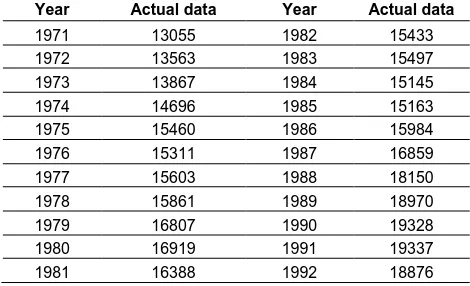
To verify the effectiveness of the proposed model, all historical enrolments in Table 1 (the enrolment data at the University of Alabama from 1971s to 1992s) are used to illustrate for forecasting process. The step-wise procedure of the forecasting model is presented as following:

Step 1: Defining the universe of discourse and intervals for observations.

Assume Y(t) be the historical data of enrolments at year t( 1971≤ 𝑡 ≤ 1992). The universe of discourse is

defined as U = [D_min , D_max]. In order to ensure the forecasting values bounded in the universe of discourse U, we set Dmin= Imin− N1 and Dmax=

I_max+ N₂; where I_min , I_max are the minimum and maximum data of Y(t); N₁and N₂ are two proper positive integers to tune the lower bound and upper bound of the U. Based on Imin and Imax, we define

the universal discourse U. From the historical data shown in Table 1, we obtain Imin= 13055 và Imax=

19337. Thus, the universe of discourse is defined as U= [ Imin− N1, Imax+ N2]= [13000,20000] with N1=

55 and N2= 663.

Now, divide the universe of discourse into n equal lengths of intervals u₁, u₂, . . . , u_n. Each interval ui of time series data set can be calculated as follows:

𝑢_𝑖= (𝐷_𝑚𝑖𝑛+ (𝑖 − 1)𝐷𝑚𝑎𝑥−𝐷𝑚𝑖𝑛

𝑛 , 𝐷𝑚𝑖𝑛+ 𝑖

𝐷𝑚𝑎𝑥−𝐷𝑚𝑖𝑛

𝑛 ]

(1)

Compared to the previous models in [2], [3], [4]. Based on Eq.(1), we cut U into seven intervals, u₁, u₂, . . . , u₇ ( 1 ≤ i ≤ n, n = 7) respectively. Thus, the seven intervals are: u1 = (13000, 14000], u2 = (14000,15000], …, u6 = (18000,19000], u7 = (19000, 20000].

TABLE I: Historical enrolments of the University of Alabama

Year Actual data Year Actual data

1971 13055 1982 15433

1972 13563 1983 15497

1973 13867 1984 15145

1974 14696 1985 15163

1975 15460 1986 15984

1976 15311 1987 16859

1977 15603 1988 18150

1978 15861 1989 18970

1979 16807 1990 19328

1980 16919 1991 19337

1981 16388 1992 18876

Step 2: Define the fuzzy sets for each observations

Assume that there are n intervals 𝑢1, 𝑢1, 𝑢1, …,𝑢𝑛

for data set obtained in Step 1. For n intervals, there are n linguistic values which are 𝐴1, 𝐴2, 𝐴3, … , 𝐴𝑛−1

and 𝐴_𝑛 to represent different regions in the universe of discourse, respectively. Each linguistic variable represents a fuzzy set 𝐴_𝑖 (1 ≤ 𝑖 ≤ 𝑛) and its definition is described in (2) .

Ai = ∑ aij

uj

𝑛

j=1 ; (2)

where a_ij∈[0,1], 1 ≤ i ≤ n, 1 ≤ j ≤ n and uj is the j-th interval. The value of a_ij indicates the grade of membership of uj in the fuzzy set Ai and it is shown as following:

1 if j == i

𝑎𝑖𝑗= 0.5 if j == i − 1 or j == i + 1

0 otherwise

(3)

From Eq.(2) and Eq.(3), each fuzzy set Ai (1 ≤ i ≤ 7) is defined as follows:

𝐴₁= 1 𝑢₁+

0.5 𝑢₂ +

0

𝑢₃+ ⋯ . + 0 𝑢₆+

(3)

Vol. 3 Issue 1, January - 2017 𝐴2=

0.5 𝑢1

+ 1 𝑢2

+0.5 𝑢3

+ ⋯ . + 0 𝑢6

+ 0 𝑢7

………....

𝐴₇= 0 𝑢₁+

0 𝑢₂+

0

𝑢₃+ ⋯ . + 0.5

𝑢₆ + 1 𝑢₇

Step 3: Fuzzify variations of the historical data (or observations)

In order to fuzzify all historical data, it’s necessary to assign a corresponding linguistic value to each interval first. The simplest way is to assign the linguistic value with respect to the corresponding fuzzy set that each interval belongs to with the highest membership degree. As in [2, 3], a historical data is fuzzified to Ai if the maximal degree of membership of that datum is in Ai.

Fuzzify(ADt) = Ai if FAD(t)(Ai) = max[FAD(t)(Ak)] for all k,

where k =1,…,ADt is the Actual data at time t; and FAD(t)(Ak)] is the degree of membership of ADt under Ak. For example, from Table 1, we can see that the actual data of year 1971 is 13055, where 13055 falls in the interval u = [13055, 14000]. Therefore, the enrolment of year 1971 (i.e., 13055) is fuzzified into 𝐴1. The

results of fuzzification are listed in Table 2, where all historical data are fuzzified to be fuzzy sets.

TABLE II: FUZZIFIED ENROLMENTS OF THE UNIVERSITY OF ALABAMA

Year

Actual data

Fuzzy

set Year

Actual data

Fuzzy set

1971 13055 A1 1982 15433 A3

1972 13563 A1 1983 15497 A3

1973 13867 A1 1984 15145 A3

1974 14696 A2 1985 15163 A3

1975 15460 A3 1986 15984 A3

1976 15311 A3 1987 16859 A4

1977 15603 A3 1988 18150 A6

1978 15861 A3 1989 18970 A6

1979 16807 A4 1990 19328 A7

1980 16919 A4 1991 19337 A7

1981 16388 A4 1992 18876 A6

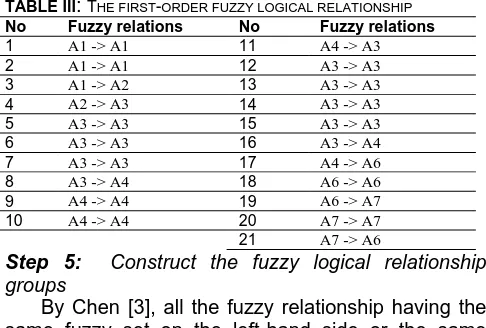
Step 4: Establishing all fuzzy logical relationships

Relationships are identified from the fuzzified historical data obtained in Step 3. If the fuzzified enrolments of years t and t - 1 are Ai and Aj, respectively, then construct the first – order fuzzy logical relationship ‘‘Ai → Aj”, where Ai and Aj are called the fuzzy set on the left-hand side and fuzzy set on the right-hand side of fuzzy logical relationships, respectively. From Table 2, we can obtain fuzzy relationships are shown in Table 3 as follows:

TABLE III: THE FIRST-ORDER FUZZY LOGICAL RELATIONSHIP No Fuzzy relations No Fuzzy relations

1 A1 -> A1 11 A4 -> A3

2 A1 -> A1 12 A3 -> A3

3 A1 -> A2 13 A3 -> A3

4 A2 -> A3 14 A3 -> A3

5 A3 -> A3 15 A3 -> A3

6 A3 -> A3 16 A3 -> A4

7 A3 -> A3 17 A4 -> A6

8 A3 -> A4 18 A6 -> A6

9 A4 -> A4 19 A6 -> A7

10 A4 -> A4 20 A7 -> A7

21 A7 -> A6

Step 5: Construct the fuzzy logical relationship groups

By Chen [3], all the fuzzy relationship having the same fuzzy set on the left-hand side or the same

current state can be put together into one fuzzy relationship group. However, the repeated FLRs are counted only once [1],[2],[3].

Suppose there are relationships such that 𝐴₁ → 𝐴₁ ; 𝐴₁ → 𝐴₂ ; 𝐴₁ → 𝐴₁;………..

We can be grouped into a relationship group as follows: 𝐴₁ → 𝐴₁, 𝐴₂…

In the weighted models [9], the recurrence of each fuzzy logical relation should be taken into account.

Suppose there are FLRs in chronological order as follows: (t= 1) 𝐴₁ → 𝐴₁

(t=2) 𝐴1 → 𝐴2

(t=3) 𝐴₁ → 𝐴₁

From this viewpoint, we can be grouped into a relationship group as follows: : 𝐴₁ → 𝐴₁, 𝐴₂, 𝐴₁,… then assign different weights for each FLR.

Based on this recurrence fuzzy logical relation and from Table 3, we get the first – order fuzzy logical relation groups are shown in Table 4.

TABLE IV: THE FIRST-ORDER FUZZY LOGICAL RELATIONSHIP GROUPS

No Relationships

1 A1 −> A1, A1, A2

2 A2 −> A3

3 A3 −> A3, A3, A3, A4, A3, A3, A3, A3, A4

4 A4 −> A4, A4, A3, A6

5 A6 −> A6, A7

6 A7 −> A7, A6

Step 6: Compute the forecasting results.

Calculate the forecasted output at time t by using the following principles:

Rule 1: If the fuzzified enrolment of year t-1 is Aj and there is only one fuzzy logical relationship in the fuzzy logical relationship group whose current state is Aj, shown as follows: A_j→ A_k ;then the forecasted enrolment of year t forecasted = mk where mk is the midpoint of the interval uk and the maximum membership value of the fuzzy set Ak occurs at the interval uk

Rule 2: If the fuzzified enrolment of year t -1 is Aj and there are the following fuzzy logical relationship group whose current state is Aj , shown as follows:

A_j→ A_i1(𝑥1), Ai2(𝑥2), … , Aip(𝑥𝑝)

then the forecasted enrolment of year t is calculated as

follows: f𝑜𝑟𝑒𝑐𝑎𝑠𝑡𝑒𝑑 =𝑥1𝑚𝑖1+𝑥2𝑚𝑖2+⋯+𝑥𝑝𝑚𝑖𝑝

𝑥1+𝑥2+⋯+𝑥𝑝 ; 𝑝 ≤ 𝑛

where 𝑚_𝑖1, 𝑚_𝑖2, … 𝑎𝑛𝑑 𝑚_𝑖𝑝 are the middle values of the intervals u1 , u2 and up respectively, and the maximum membership values of A1, A2 , . .. ,Ap occur at intervals u1 , u2,…, up , respectively; 𝑥₁, 𝑥₂,… and 𝑥𝑝 notes the number of fuzzy logical relationships

‘‘𝐴_𝑗→ 𝐴_𝑖𝑘”, (1≤ 𝑘 ≤p) in the fuzzy logical relationship group.

(4)

Vol. 3 Issue 1, January - 2017 where the symbol ‘‘#” denotes an unknown value,

then the forecasted enrollment of year t + 1 is 𝑚_𝑗, where 𝑚𝑗 is the midpoint of the interval 𝑢𝑗 and the

maximum membership value of the fuzzy set 𝐴_𝑗, occurs at 𝑢_𝑗.

From these rules, we can obtain these forecasting results are listed in Table 5.

TABLE V: FORECASTED ENROLMENTS OF UNIVERSITY OF ALABAMA BASED ON THE FIRST – ORDER FTS MODEL.

Year Actual Fuzzified Results

1971 13055 A1 Not forecasted

1972 13563 A1 14000

1973 13867 A1 14000

1974 14696 A2 14000

1975 15460 A3 15500

1976 15311 A3 15788.9

1977 15603 A3 15788.9

1978 15861 A3 15788.9

1979 16807 A4 15788.9

1980 16919 A4 17000

1981 16388 A4 17000

1982 15433 A3 17000

1983 15497 A3 15788.9

1984 15145 A3 15788.9

1985 15163 A3 15788.9

1986 15984 A3 15788.9

1987 16859 A4 15788.9

1988 18150 A6 17000

1989 18970 A6 19166.7

1990 19328 A7 19166.7

1991 19337 A7 18833.3

1992 18876 A6 18833.3

1993 N/A # 19166.7

B. Adjusted the forecasting results by Fourier series

In order to improve the accuracy of forecasting models, the Fourier series has been successfully applied in modifying the residuals in fuzzy time series model which reduces the forecasting values.

The procedure to obtain the modified residuals from fuzzy time series forecasting model with Fourier series is as the following.

Suppose an original series (the historical data series at time t ) with n entries is Y_t= {x₁(t), x2(t), … , xn(t)}

and its predicted series (forecasting value at time t), under weighted fuzzy time series is Ŷ =_t {x̂ (t), x1 ̂(t), … , x2 ̂(t)n } then, its residual series is

defined as: 𝛆 = [𝜀1, 𝜀2, … , 𝜀𝑡], with 𝑡 = 1, 𝑛̅̅̅̅̅.

The analysis process for the residual series are derived as follows:

𝛆𝐭= 𝐘𝐭− 𝐘̂ 𝐭 (4)

Now, let’s consider a sub-series

𝛆

∗

_as:

𝛆

∗_{= [𝜀}

2, 𝜀3, … , 𝜀𝑡… , 𝜀𝑡], with 𝑡 = 2, 𝑛̅̅̅̅̅ (5)

Based on Table 6, we get the residual series between actual value and forecasting value as follows:

ε_t= (−437, −113, . . . ,503, 42.7)_1𝑥21 And

𝛆

∗=

(

−113, 696, . . . ,503, 42.7

)

_1𝑥20

Following, Fourier series transform can be used to latch the implied periodic phenomenon in the residual series. Then, using Fourier modification technique in

residual analysis, we can rise forecasting performance from the considered input data set. The estimated residual series can be modeled by Fourier series transform as follows:

𝛆̂ = _𝐭 1

2𝑎0+ ∑ [𝑎𝑖cos( 2𝜋𝑖 𝑛−1𝑡) 𝑑

𝑖=1 + 𝑏𝑖sin(

2𝜋𝑖

𝑛−1𝑡)], with 𝑡 =

1, 𝑛

̅̅̅̅̅ (6)

Where: 𝑑 =𝑛−1

2 is called the minimum deployment

frequency of Fourier series [19] and only take integer number. And therefore, the residual

sub-series

is rewritten as:

𝛆∗_{= 𝑷 ∗ 𝑪} ₍₇₎

Where:

𝐶 = (𝑎₀, 𝑎₁, 𝑏₁… 𝑎_𝑑, 𝑏_𝑑)

P = (⌊1

2⌋_(n−1)x1p1… Pk… Pd) , with 𝑃𝑘 is

determined by Eq.(8) as follows:

𝑷_𝒌=

[

cos (2𝜋 ∗ 2 ∗ 𝑘

𝑛 − 1 ) sin (

2𝜋 ∗ 2 ∗ 𝑘 𝑛 − 1 )

cos (2𝜋 ∗ 3 ∗ 𝑘

𝑛 − 1 ) sin (

2𝜋 ∗ 3 ∗ 𝑘 𝑛 − 1 ) ⋮ ⋮

cos (2𝜋 ∗ 𝑛 ∗ 𝑘

𝑛 − 1 ) sin (

2𝜋 ∗ 𝑛 ∗ 𝑘 𝑛 − 1 )]

𝑤ℎ𝑒𝑟𝑒 , 𝑘 = 1, 𝑑̅̅̅̅̅

The parameters a₀, a₁, b₁, … , a_d, b_d are obtained by using the ordinary least squares method (OLS) which results in the Eq.(8) as following:

𝐂 = (𝐏𝐓_𝐏)−𝟏_𝐏𝐓_𝛆∗𝐓 ₍₈₎

From value of ε∗_{and value of matrix P, we calculate}

the parameters as following:

C = (5.13, 36.87, −113, . . . , −5.30, −130)1𝑥21

Next, Once the parameters are calculated, the forecasting series residual 𝜀(𝑡)̂ is then easily achieved based on the Eq.(6). Therefore, based the predicted series Ŷ_t obtained from weighted fuzzy time series model, the forecasting series 𝛆′̂_𝐭 of the modified model is determined by:

𝛆′̂ = [𝜺𝐭 ̂ 𝜺𝟏, ̂, 𝜺𝟐 ̂, … , 𝜺𝟑 ̂ ] 𝒏 (9)

Where , { 𝜺′̂ = x𝟏 ̂1

𝛆′̂ = 𝐘𝐭 ̂ + 𝜺(𝒕) , 𝑤𝑖𝑡ℎ 𝑡 = 2, 𝑛𝐭 ̅̅̅̅̅

From Eq.(9) and based on Table 5, we get the finally forecasting results in 5-th columns of Table 6 after adjusted residual series.

TABLE VI: FORECASTED ENROLMENTS OF UNIVERSITY OF ALABAMA BASED ON WEIGTH FTS MODEL AND FOURIER SEIRIES TRANSFORM.

Year Actual Fuzzified Weigth FTS model Modified model

1971 13055 A1 - -

1972 13563 A1 14000 -

1973 13867 A1 14000 13864

1974 14696 A2 14000 14693

(5)

1976 15311 A3 15788.9 15308

1977 15603 A3 15788.9 15600

1978 15861 A3 15788.9 15858

1979 16807 A4 15788.9 16804

1980 16919 A4 17000 16916

1981 16388 A4 17000 16385

1982 15433 A3 17000 15430

1983 15497 A3 15788.9 15494

1984 15145 A3 15788.9 15142

1985 15163 A3 15788.9 15160

1986 15984 A3 15788.9 15981

1987 16859 A4 15788.9 16856

1988 18150 A6 17000 18147

1989 18970 A6 19166.7 18967

1990 19328 A7 19166.7 19325

1991 19337 A7 18833.3 19334

1992 18876 A6 18833.3 18873

1993 N/A # 19166.7 18965

IV. EXPERIMENTAL RESULTS

Experimental results for our model will be compared with the existing methods, such as the SCI model [2], the C96 model [3], the S.R.Singh model [7] and the H01 model [5] by using the enrolment of Alabama University from 1972s to 1992s are listed in Table 7 .

To evaluate the forecasted performance of proposed method in the FTS, the mean square error (MSE) and the mean absolute percentage error (MAPE) are used as a comparison criterion to represent the forecasted accuracy. The MSE value and MAPE value are computed according to (10) and (11) as follows:

MSE = 1

n∑ (Fi− Ri) 2 n

i=1 (10)

𝑀𝐴𝑃𝐸 = 1

𝑛∑ |

𝐹𝑖−𝑅𝑖

𝑅𝑖 |

𝑛

𝑖=1 ∗ 100% (11)

Where, Ri notes actual data on year i, Fi forecasted

value on year i, n is number of the forecasted data Table 7 shows a comparison of MSE and MAPE of our method using the first-order FTS under different number of intervals, where MSE and MAPE are calculated according to (10) and (11) as follows:

𝑀𝑆𝐸 = ∑20𝑖=1(𝐹𝑖−𝑅𝑖)2

𝑁 =

(13864−13867)2_{+(14693−14696)}2_{…+(18873−18876)}2

20 = 8.57

𝑀𝐴𝑃𝐸 = 1

20∑ |

𝐹𝑖−𝑅𝑖

𝑅𝑖 |

20

𝑖=1 ∗ 100% =

1 20(

𝑎𝑏𝑠(13864−13563)

13563 +

⋯ +𝑎𝑏𝑠(18873−18876)

18876 ) = 0.0175%

where N denotes the number of forecasted data, Fi denotes the forecasted value at time i and Ri denotes the actual value at time i.

TABLE VII: A COMPARISON OF THE FORECASTED RESULTS OF PROPOSED MODEL WITH THE EXISTING MODELS BASED ON THE SECOND-ORDER FUZZY TIME SERIES BY ADJUSTING FOURIER SEIRIES.

Year Actual data SCI C96 H01 S.R.Singh Our model

1971 13055 - - - -

1972 13563 14000 14000 14000 -

1973 13867 14000 14000 14000 13864

1974 14696 14000 14000 14000 14500 14693

1975 15460 15500 15500 15500 15358 15457

1976 15311 16000 16000 15500 15500 15308

1977 15603 16000 16000 16000 15500 15600

1978 15861 16000 16000 16000 15500 15858

1979 16807 16000 16000 16000 16500 16804

1980 16919 16813 16833 17500 16500 16916

1981 16388 16813 16833 16000 16500 16385

1982 15433 16789 16833 16000 15581 15430

1983 15497 16000 16000 16000 15500 15494

1984 15145 16000 16000 15500 15500 15142

1985 15163 16000 16000 16000 15500 15160

1986 15984 16000 16000 16000 15500 15981

1987 16859 16000 16000 16000 16402 16856

1988 18150 16813 16833 17500 18500 18147

1989 18970 19000 19000 19000 18500 18967

1990 19328 19000 19000 19000 19471 19325

1991 19337 19000 19000 19500 19500 19334

1992 18876 19000 19000 19149 19651 18873

MSE 423027 407507 226611 115972 8.57

MAPE 3.22% 3.11% 2.66% 1.71% 0.0175%

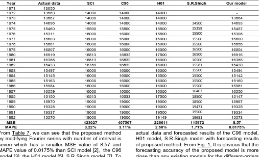
From Table 7, we can see that the proposed method by modifying Fourier series with number of interval is seven which has a smaller MSE value of 8.57 and MAPE value of 0.0175% than SCI model [2], the C96 model [3], the H01 model [5], S.R Singh model [7]. To be clearly visualized, Fig. 1 depicts the trends for

actual data and forecasted results of the C96 model, H01 model, S.R.Singh model with forecasting results of proposed method. From Fig. 1, It is obvious that the forecasting accuracy of the proposed model is more close than any existing models for the different-orders

(6)

Fig. 1: The curves of the C96, H01, S.R.Singh models and our model for forecasting enrolments of University of Alabama

V. CONCLUSIONS

In this paper, we have presented a hybrid forecasted method to handle forecasting enrolments of the University of Alabama based on which combines the weighted fuzzy time series and Fourier series techniques. Firstly, we propose weighted models to tackle two issues in fuzzy time series forecasting, namely, recurrence and weighting. Based on forecasted result obtained. Then, we use Fourier series to modify the residuals of the weighted FTS for improving the forecasting performance. Next, we calculate forecasting output and compare forecasting accuracy with other existing models. Lastly, based on the performance comparison in Tables 7 and Fig. 1, it can show that our model outperforms previous forecasting models with various orders and the same interval length.

The proposed model was only tested by the forecasting enrollment problem, and it can actually be applied to other practical problems such as population forecast, and rice production forecasting in the further research.

REFERENCES

[1] Q. Song, B.S. Chissom, “Forecasting Enrollments with Fuzzy Time Series – Part I,” Fuzzy set and system, vol. 54, pp. 1-9, 1993b.

[2] Q. Song, B.S. Chissom, “Forecasting Enrollments with Fuzzy Time Series – Part II,” Fuzzy set and system, vol. 62, pp. 1-8, 1994.

[3] S.M. Chen, “Forecasting Enrollments based on Fuzzy Time Series,” Fuzzy set and system, vol. 81, pp. 311-319. 1996.

[4] Hwang, J. R., Chen, S. M., & Lee, C. H. Handling forecasting problems using fuzzy time series. Fuzzy Sets and Systems, 100(1–3), 217–228, 1998.

[5] Huarng, K. Heuristic models of fuzzy time series for forecasting. Fuzzy Sets and Systems, 123, 369–386, 2001b .

[6] Singh, S. R. A simple method of forecasting based on fuzzy time series. Applied Mathematics and Computation, 186, 330–339, 2007a.

[7] Singh, S. R. A robust method of forecasting based on fuzzy time series. Applied Mathematics and Computation, 188, 472–484, 2007b.

[8] S. M. Chen, “Forecasting enrollments based on high-order fuzzy time series”, Cybernetics and Systems: An International Journal, vol. 33, pp. 1-16, 2002.

[9] H.K.. Yu “Weighted fuzzy time series models for TAIEX forecasting ”, Physica A, 349 , pp. 609–624, 2005. [10] Chen, S.-M., Chung, N.-Y. Forecasting enrollments of

students by using fuzzy time series and genetic algorithms. International Journal of Information and Management Sciences 17, 1–17, 2006a.

[11] Chen, S.M., Chung, N.Y. Forecasting enrollments using high-order fuzzy time series and genetic algorithms. International of Intelligent Systems 21, 485–501, 2006b. [12] Huarng, K. theH. Effective lengths of intervals to improve

forecasting fuzzy time series. Fuzzy Sets and Systems, 123(3), 387–394, 2001a.

[13] Lee, L.-W., Wang, L.-H., & Chen, S.-M. Temperature prediction and TAIFEX forecasting based on fuzzy logical relationships and genetic algorithms. Expert Systems with Applications, 33, 539–550, 2007.

[14] Jilani, T.A., Burney, S.M.A. A refined fuzzy time series model for stock market forecasting. Physica A 387, 2857–2862. 2008.

[15] Wang, N.-Y, & Chen, S.-M. Temperature prediction and TAIFEX forecasting based on automatic clustering techniques and two-factors high-order fuzzy time series. Expert Systems with Applications, 36, 2143–2154, 2009 [16] Kuo, I. H., Horng, S.-J., Kao, T.-W., Lin, T.-L., Lee, C.-L.,

& Pan. An improved method for forecasting enrollments based on fuzzy time series and particle swarm optimization. Expert Systems with applications, 36, 6108–6117, 2009a.

[17] S.-M. Chen, K. Tanuwijaya, “ Fuzzy forecasting based on high-order fuzzy logical relationships and automatic clustering techniques”, Expert Systems with Applications 38 ,15425–15437, 2011.

[18] Shyi-Ming Chen, Nai-Yi Wang Jeng-Shyang Pan. Forecasting enrollments using automatic clustering techniques and fuzzy logical relationships, Expert Systems with Applications 36 , 11070–11076, 2009. [19] Y. L. Huang and Y. H. Lee, Accurately forecasting

model for the Stochastic Volatility data in tourism demand, Modern Econ. 2, pp. 823-829, 2011.

1972 1974 1976 1978 1980 1982 1984 1986 1988 1990 1992 1.3