Efficient Formulations for 1-SVM and their
Application to Recommendation Tasks
Yasutoshi Yajima and Tien-Fang Kuo
Department of Industrial Engineering and Management, Tokyo Institute of Technology, Japan Email:{yasutosi,kuo}@me.titech.ac.jp
Abstract— The present paper proposes new approaches for recommendation tasks based on one-class support vector machines (1-SVMs) with graph kernels generated from a Laplacian matrix. We introduce new formulations for the 1-SVM that can manipulate graph kernels quite efficiently. We demonstrate that the proposed formulations fully utilize the sparse structure of the Laplacian matrix, which enables the proposed approaches to be applied to recommendation tasks having a large number of customers and products in practical computational times. Results of various numerical experiments demonstrating the high performance of the proposed approaches are presented.
Index Terms— support vector machine, Laplacian matrix, graph kernel, quadratic programming problem, collabora-tive filtering, recommender system
I. INTRODUCTION
Recently, the importance of recommender systems has increased rapidly with the growing availability of online information on the Web. Customers visiting the largest e-commerce sites often have difficulty in finding a particular item among the enormous number of products for sale. Many recommender systems [1], [2] have been installed to filter out irrelevant products and locate products that might be of interest to individual customers.
Collaborative filtering is one of the most successful technologies for recommendation tasks, in which cus-tomer ratings on products or historical records of pur-chased products are exploited to extract the preferences of individuals. Collaborative filtering calculates similarities between customers based on the customer rating, or the purchased products patterns of each individual. Collabo-rative filtering then finds a set of the most similar patterns, and recommends products for a particular individual. In the present paper, we provide new approaches for recom-mendation tasks using kernelsdefined on a graph where the nodes correspond to data items such as the products, and the weights of the edges correspond the relations between the products. There have been several graph based kernels which can be used to obtain similarities between data points.
Very recently, Fouss et al. [3] introduced a graph kernel, referred to as the commute time kernel and directly applied the kernel-based dissimilarities to the recommen-dation task. More precisely, they defined the kernel over
This paper is based on “One-Class Support Vector Machines for Rec-ommendation Tasks,” by Y. Yajima, which appeared in the Proceedings of the 10th Pacific-Asia Conference on Knowledge Discovery and Data Mining (PAKDD 2006), Singapore, April 9-12, 2006.
a bipartite graph with two sets of nodes corresponding to a set of customers and products. They placed edges between the customer nodes and the product nodes when the customer has purchased the product. They defined a random walk model over this graph by assigning the transition probabilities over the edges. They showed that the average commute time between the two nodes is given by the kernel and that it can be used as a distance measure between the corresponding customer and product.
In the present paper, we use the 1-SVM with graph-based kernels to select relevant products for each cus-tomer. We introduce new formulations for the 1-SVM that can efficiently manipulate several recently developed graph kernels, such as [4], [5], [6], [7]. In addition, we show that a special case of our formulation does not require any optimization calculations. More importantly, the new kernel matrix is significantly smaller than that of the method reported in [3], which enables us to apply the present approach to large e-commerce sites with a practical amount of computation.
In Sect. II, we briefly review the standard formulation of the 1-SVM and its basic settings for recommendation tasks. In Sect. III, we describe various graph kernels, and in Sect. IV, we introduce new formulations for the 1-SVM. Experiments using a movie dataset are presented in Sect. V, and conclusions are presented in Sect. VI.
II. 1-SVMFORRECOMMENDATION
The SVM was originally designed as a method for two-class classification problems where both positive and negative examples are required to learn discriminate func-tions. In this section, we will describe a variant of the SVM, called the one-class SVM (1-SVM) which can handle problems that consider a single class of data points. In [8], Sch ¨olkopf et al. have proposed a method for adapting the conventional two-class SVM formulation to the one-class problems.
Suppose that we have a set of N-dimensional data pointsxj ∈ RN (j = 1,2, . . . , l). Also, assume that we have a functionφ(·) :RN → F that maps the data points into a higher-dimensional feature space, denoted by F. Hereinafter, for simplicity, we denote the mapped image
Introducing additional variablesξ = (ξ1, ξ2, . . . , ξl)T, w andρare obtained by solving the following quadratic programming problem:
Min. 12w,w+ 1 νl
l
j=1ξj−ρ
s.t. w , φj+ξj ≥ρ, ξj≥0, j= 1,2, . . . , l,
(1) where ν ∈ (0,1] is a predetermined positive parameter. Let (w∗, ρ∗)denote an optimal solution of the problem (1). When a data point, the mapped image of which is denoted by φ, belongs to the negative side of the hyperplane, i.e., w∗, φ −ρ∗ <0, the pattern can be considered to be different from the given single class of data points.
The objective of the recommendation task is to find products that have not yet been purchased but that would likely be purchased by a specific customer, hereinafter referred to as an active customer. Suppose that we are given a set of products P = {1,2, . . . , M} and that, for each product j ∈ P, the associated feature vectors
φj ∈ F are obtained. In addition, let P(a) ⊆ P be a subset of indices that are rated as preferable products, or that have actually been purchased by the active customer
a. For simplicity, let us assume that P(a) consists of l
products and is denoted as P(a) = {1,2, . . . , l}, which is treated as a set of the single class of data points in the problem (1). Let (w∗, ρ∗) denote an optimal solution of (1). Then, for each productithat has not been purchased, i.e., i ∈ P \ P(a), the distance from the hyperplane calculated as (w∗, φi −ρ∗)/w∗,w∗ can be used as a preference score of the product i. Ignoring the constants, one can use the inner product w∗, φias a scoreto rank the productifor the specific active customer
a. It has been shown that the parameterν enjoys theν -property[8] described below:
Theorem 1: νis an upper bound on the fraction of the data points lying in the negative side of the hyperplane. Also, ν is a lower bound on the fraction of the data points lying in the nonnegative side of the hyperplane, i.e.,w∗, φi −ρ∗≥0.
Generating a nonlinear map φ(·) is quite important in SVM. Usually, this is done implicitly bykernelsthat are naturally introduced by the following dual formulation of the problem (1).
Max. −1 2
l
i=1
l
j=1φi, φjαiαj
s.t. lj=1αj= 1, 0≤αj≤ νl1, j= 1,2, . . . , l,
(2) where α1, α2,· · ·, αl are dual variables. Note that the dual formulation can be defined using only the values of the inner products, without knowing the mapped image
φi, explicitly. In addition, let (α∗1, α∗2,· · · , α∗l) be an optimal solution of the dual problem. Then, the associated optimal primal solution is given as w∗ = lj=1α∗jφj, which immediately implies that the score of the product
iis given byw∗, φi=jl=1α∗jφi, φj.
LetK={Kij}be a symmetric matrix called a kernel matrix, which consists of the inner productsφi, φjas thei−j element. Any positive semidefinite matrices can
be used as a kernel matrixK. It has been shown that posi-tive semidefiniteness ensures the existence of the mapped points, φi’s (see, for example, [9]). More precisely, let
U be an orthonormal matrix whose columns correspond to the eigenvectors of K, and Λ be a diagonal matrix whose diagonal elements correspond to the eigenvalues of K. When the matrix K is positive semidefinite, one can obtain the eigendecomposition K = UΛUT. Then, the mapped imageφiis explicitly given as theith column vector of the matrix Λ12UT, i.e.,
Λ12UT = [φ1φ2· · ·φl]. (3) In the next section, we will introduce recently devel-oped kernel matrices defined on the graph.
III. LAPLACIAN OF AGRAPH ANDASSOCIATED KERNEL
Recently, several studies [4], [5], [6], [7] have reported the development of kernels using weighted graphs. In this section, we will review such kernels.
First, let us introduce a weighted graphG(V, E)having a set of nodes V and a set of undirected edges E. The set of nodesV corresponds to a set of data items such as products in a recommendation task. For each edge(i, j)∈
E, a positive weight bij >0 representing the similarity between the two nodesi, j ∈V is assigned. We assume that the larger the weight bij, the greater the similarity between the two nodes. Note that if there exists no edge betweeniandj, then we setbij= 0.
The edge weightsbij’s are defined in several ways. For example, the following exponential function is often used
bij = exp
− xi−xj 2
σ2
, (4)
whereσis a bandwidth hyperparameter. One can also use ak-nearest-neighbor graph where we put an edge between the nodeiandj when the data pointxi is among the k
nearest neighbors ofxj or vice versa, and assign a weight
bij as (4), or, simply,bij = 1for each edge(i, j). LetM
be the number of nodes in V, and letB be an M ×M
symmetric matrix with elementsbij for(i, j)∈E.
Next, let us introduce the Laplacian matrix L of the graph G(V, E) as L = D−B, whereD is a diagonal matrix, the diagonal elements dii of which are the sum of the ith row of B, i.e., dii =jbij. Throughout this paper, we assume that the graph G(V, E) is connected. This implies that the rank of the matrix L is M −1, and that the null space ofLis the one-dimensional space spanned by the vector of all ones, i.e.,Le= 0.Also, It has been known thatL is positive semidefinite (see [10] for further details).
There are several methods for generating kernel matri-ces based on L. Fouss et al. [3] considered a random walk model on the graph G, in which, for each edge (i, j), the transition probability pij is defined as pij =
bij/Mk=1bik. Intuitively, at each node i, the transition probability to the node j is proportional to the weight
which represents the average number of steps that a random walker, starting from node i, will take to enter nodej for the first time and then return to nodei. They indicated that the average commute time n(i, j) can be used as a dissimilarity measure between any two data points corresponding to the nodes of the graph, and that
n(i, j)is given asn(i, j) =VGlii++ljj+−2lij+,where
VG=i,jbij andl+ij is thei−j element of the Moore-Penrose pseudoinverse of L, which is denoted by L+. Fouss et al. [3] also showed that as long as the graph is connected, the pseudoinverseL+ is explicitly given as follows:
L+=L−eeT/M−1+eeT/M, (5) where e is a vector of all ones. Since L is positive semidefinite [10], so is its pseudoinverse L+, which
implies thatL+ can act as a kernel matrix [3].
Here, L and L+ share the common eigenvectors. Let v1,v2, . . . ,vM and λ1, λ2, . . . , λM be the eigenvectors
and the corresponding eigenvalues of L, respectively. It is well-known that L is decomposed into L =
M
i=1λi(vivTi), and that the pseudoinverse is also given
as
L+=
M
i=1
λ+i (vivTi ), where λ+=
λ−1 ifλ= 0 0 ifλ= 0.
(6) We note that
L+e= 0. (7)
Several variants of the above equation have been pro-posed. Zhuet al.[11] introduced the following regularized Laplacian kernel matrix
M
i=1
(1+tλi)−1vivTi =
∞
k=0
tk(−L)k= (I+tL)−1. (8)
Moreover, by introducing the modified Laplacian Lr =
rD−Bwith a parameter0≤r≤1, Itoet al.[7] defined the modified Laplacian regularized kernel matrix as
(I+tLr)−1. (9)
In particular, when r = 0 this kernel matrix is the von Neumann diffusion kernel, which is defined as
∞
k=0
tkBk = (I−tB)−1. (10)
Furthermore, introducing the normalized Laplacian ˜
L ≡ D−1/2LD−1/2, Smola and Kondor [5] proposed
several kernel matrices such as the diffusion kernel
exp(−tL˜) (11)
and a normalized variant of the regularized Laplacian kernel defined as follows:
I+tL˜
−1
. (12)
IV. LEARNING1-SVMS WITHGRAPHKERNELS Next, we will describe recommendation methods based on the 1-SVM using the kernel matrices described in the previous section. Recall that we are given a set of M
products P = {1,2, . . . , M} and a subset P(a) ⊆ P, which have been purchased by the active customera. We assume that P(a) = {1,2, . . . , l}. In addition, the ele-ments of the kernel matrixKrepresent the inner products of the feature vectors corresponding to the products.
Let us first rewrite the primal formulation. To this end, introducingM variablesα= (α1, α2,· · · , αM)T,let us assume that w ∈ F is given as a linear combination of
M points as follows:
w=
M
j=1 αjφj.
Substituting this equation into the primal problem (1), the following formulation is obtained:
Min. 12αTKα+νl1 li=1ξi−ρ
s.t. Mi=1αiφi, φj
+ξj≥ρ, j= 1,2, . . . , l, ξj ≥0, j= 1,2, . . . , l.
(13) Note that the norm of w can be written as follows:
w,w=
M
j=1 αjφj,
M
j=1 αjφj
=αTKα.
Let α∗ = (α∗1, α∗2, . . . , α∗M)T be an optimal solution of
this problem. Then, the preference score of the producti
is given as theith element of the vectorKα∗, i.e.,
M
j=1
α∗jφi, φj
= (Kα∗)i. (14)
Here, generating the kernel matrices given in Sect. III requires calculation of the inverse of the matrices as described in (5) and (8). The inverse operations require a significant computational effort, which prevents us from using these kernel matrices for the recommendation tasks when the number of products is large. Moreover, in general, these kernel matrices become fully dense, which causes difficulty in holding the kernel matrices in memory during the time required for solving the problem (13). In the subsequent subsections, however, we will propose new formulations of 1-SVMs with kernel matrices the inverse of which are readily available. Exploiting the special structures of the kernel matrices, we will derive simpler formulations for solving 1-SVM with the kernel matrices (5) and (8).
A. Regularized Laplacian Kernel
Suppose that the kernel matrix K is the regularized Laplacian kernel matrix (8). Let us first introduce a new vector of variables β = (β1, β2, . . . , βM)T ∈ RM, and defineβ≡Kα. Note that
βj= (Kα)j=
M
i=1
αiφi, φj
holds for eachj. It follows that
α=K−1β= (I+tL)β
holds. Furthermore, a straightforward calculation reveals that
αTKα=βT(I+tL)β.
Therefore, the problem (13) can be equivalently formu-lated with respect to the new variableβ as follows:
Min. 12βT(I+tL)β−ρ+ 1 νl
l
i=1ξi
s.t. βj+ξj≥ρ, ξj ≥0, j= 1,2, . . . , l. (15)
Associated with this formulation, we have the following theorem.
Theorem 2: The problem (15) has an optimal solution (β∗,ξ∗, ρ∗)which satisfies
0≤β∗j ≤ρ∗, j= 1,2, . . . , M.
Proof: By the Karush–Kuhn–Tucker (KKT) con-ditions, there exist nonnegative Lagrangian multipli-ers vj (j = 1, . . . , l) such that the optimal solution (β∗, ρ∗,ξ∗)satisfies
((I+tL)β∗)j =
vj, ∀j= 1,2, . . . , l,
0, ∀j=l+ 1, l+ 2, . . . , M,
(16) and the complementarity conditions
vjβ∗j +ξj∗−ρ∗= 0, ∀j= 1,2, . . . , l. (17) Moreover, we note that any optimal solutions must satisfy the following
ξi∗= max{0, ρ∗−βi∗}, ∀i= 1,2, . . . , l. (18) It follows from the definition of the Laplacian matrix
L that the left hand side of (16) can be written in the following way:
((I+tL)β∗)j=βj∗+t M
i=1
bjiβj∗−βi∗,
which is nonnegative. This holds true for an index k
attaining the minimum of βj∗’s
k≡argmin{βj∗|j= 1,2, . . . , M}.
Therefore, since tis a positive parameter,
β∗k ≥ −t M
i=1
bki(βk∗−β∗i)≥0,
which implies that βj∗ is nonnegative for all j = 1,2, . . . , M, and thatρ∗≥0.
Next, on the contrary, let us assume that there exists an indexhsuch thatβh∗> ρ∗.Without loss of generality, we also assume that
h≡argmax{βj∗|j= 1,2, . . . , M}.
It follows that
((I+tL)β∗)h=β∗h+t M
i=1
bhi(βh∗−βi∗)>0. (19)
From the KKT conditions (16), the index should beh≤l, which implies that the associated Lagrangian multiplier is positive((I+tL)β∗)h=vh>0.
It follows from (18) that, however, we have ξh∗ = 0,
which results in
βh∗+ξh∗−ρ∗>0.
This contradicts the complementarity conditions (17), which completes the proof.
It follows from this theorem and the conditions (18) that the optimal solution satisfies the following equalities:
ξj=ρ−βj, j= 1,2, . . . , l.
Substituting ξj into the problem (15), we then have a simpler formulation given below:
Min. 12βT(I+tL)β+1−νν ρ−νl1 li=1βi
s.t. βj ≤ρ, j= 1,2, . . . , l. (20)
In many practical situations, the Laplacian matrix L is very sparse and can be stored in main memory even if the number of data points is very huge. Moreover, it has been shown that this problem can be equivalently optimized by solving an unconstrained minimization problemusing an implicit Lagrangian function. A more detailed description can be found in [12].
B. Commute Time Kernel
Let us consider the case when we use the commute time kernel matrixL+ asK in (13), i.e.,
Min. 12αTL+α+ 1 νl
l
i=1ξi−ρ
s.t. (L+α)
j+ξj≥ρ, j= 1,2, . . . , l, ξj ≥0, j= 1,2, . . . , l.
(21)
We will also show that a simpler formulation can be derived.
First, let (α∗, ρ∗,ξ∗) be an optimal solution of (21). It follows from (7) that, for any real numberθ ∈R, we have
L+(α∗+eθ) =L+α∗.
This implies that the solution (α∗ +eθ, ρ∗,ξ∗) is also optimal. Thus, there exists an optimal solution satisfying the following equality constraint
eTα= 1, (22)
which can be added to the problem (21).
Next, as in the previous section, let us introduce a vector of variables β = (β1, β2, . . . , βM)T, and let us define
β≡L+−eeT/Mα+e/M. (23) For eachj, if αsatisfies the added constraint (22), then
βj= L+α− e Me
Tα+ e M
j=
L+αj
=
M
i=1
αiφi, φj
holds. Therefore, it follows from (5) and (23) that
α=
L−ee T M
β− e
M
(24)
holds. In addition, we can easily verify that the constraint (22) is written as
eTα=eTL−eeT M
β− e
M
=−eT β− e
M
= 1.
Then the variableβhas to satisfyeTβ= 0. Furthermore, αTL+α = βTLβ holds if β satisfies eTβ = 0.
Therefore, the problem (21) with the constraint (22) can be equivalently formulated as follows:
Min. 12βTLβ−ρ+νl1 li=1ξi
s.t. βj+ξj≥ρ, ξj ≥0, j= 1,2, . . . , l,
eTβ= 0.
(25)
Let(β∗,ξ∗, ρ∗)be an optimal solution of the problem (25). We have the following theorem.
Theorem 3: The optimal solution(β∗,ξ∗, ρ∗)satisfies
β∗j ≤ρ∗ for allj = 1, . . . , M. Proof: Let
¯
β ≡maxβ∗j |j= 1,2, . . . , M.
For the purpose of contradiction, let us assume that β >¯ ρ∗. We will show that a better solution can be constructed. LetI be a set of indices of the vectorβ∗ defined as
I≡i|βi∗= ¯β.
Note that any optimal solutions must satisfy the following
ξi∗= max{0, ρ∗−βi∗}, ∀i= 1,2, . . . , l. (26) This implies that ξi∗ = 0 for any i ∈ I. Then, for a sufficiently small > 0, let us define a new solution
ˆ
β= ( ˆβ1,β2,ˆ · · ·,βˆM),where
ˆ
βi =
¯
β− ifi∈I
βi∗+M−|I||I| otherwise
It is obvious to see thatβˆ satisfieseTβˆ = 0. Also, when
satisfies
0< ≤ρ∗−β,¯
ˆ
βi +ξi∗ ≥ ρ∗ still hold true for all i = 1,2, . . . , l. Therefore, the point ( ˆβ,ξ∗, ρ∗) is a feasible solution of the problem (25).
On the other hand, it follows from the definition of the matrixL, we have
1 2β
∗TLβ∗−1
2 ˆ βTLβˆ
= i∈I j∈I bij
( ¯β−βj∗)2−( ¯β−βj∗− M M− |I|)
2
>0,
which implies that the solution( ˆβ,ξ∗, ρ∗)yields a better objective function value than that of (β∗,ξ∗, ρ∗)when
satisfies
0< <min
ρ∗−β,¯ M − |I| M ( ¯β−β
∗ j)
, j∈I,
which is a contradiction.
From Theorem 3 and (26), we can claim that the optimal solution(β∗,ξ∗, ρ∗)of the problem(25)satisfies
βj∗+ξj∗=ρ∗, ∀j= 1,2, . . . , l.
Consequently, by substituting ξj =ρ−βj, the problem (25) can be simplified as follows:
Min. 12βTLβ+1−νν ρ−νl1 li=1βi
s.t. βj ≤ρ, j= 1,2, . . . , l,
eTβ= 0,
(27)
which is also reduced into anunconstrained minimization problemusing an implicit Lagrangian function [12].
C. Some Special Cases
It has been shown that the 1-SVM formulation given in (1) can be solved analytically whenν= 1.0. This is also true for our formulation given in (13) with any types of kernel matrices given in Sect. III. We have the following theorem:
Theorem 4: Let(α∗,ξ∗, ρ∗)be an optimal solution of (13)with ν= 1.0, i.e.,
Min. 12αTKα+1 l
l
j=1ξj−ρ
s.t. Mi=1αiφi, φj
+ξj≥ρ, j= 1,2, . . . , l, ξj ≥0, j= 1,2, . . . , l.
(28) Then, the following inequalities hold true.
M
i=1
α∗iφi, φj
≤ρ∗, ∀j= 1,2, . . . , l.
Proof: Let us assume, to the contrary, that there exists an index k such that Mi=1α∗iφi, φk
> ρ∗. It should be noted thatξk∗= 0.
Next, let ∆ ≡ Mi=1α∗iφi, φk
−ρ∗ > 0. Then, we can define a new solution ˆξ = ( ˆξ1, . . . ,ξˆl)and ρˆ as follows:
ˆ
ξj=
ξj∗+ ∆ if j=k,
ξk∗ if j=k, and ρˆ=ρ ∗+ ∆.
It is straightforward to verify that the solution(α∗,ˆξ,ρˆ) also satisfies the constraints of the problem (28). In particular, we note that the equality
M
i=1
α∗iφi, φk
+ ˆξk = ˆρ
holds true because ξˆk= 0.
The objective value of the solution(α∗,ξˆ,ρˆ)is calcu-lated as
1 2α
∗TKα∗+1 l
l
j=1
ˆ
ξj−ρˆ
= 1 2α
∗TKα∗+1 l
j=k
(ξj∗+ ∆) +1
lξ ∗
k−ρ∗−∆
= 1 2α
∗TKα∗+1 l
l
j=1
which contradicts the optimality of the solution (α∗,ξ∗, ρ∗). This completes the proof.
This theorem also ensures that
ξj∗=ρ∗−
M
i=1
α∗iφi, φj
holds for each j = 1,2, . . . , l. Then, substituting these equations into the objective function of the problem (28), the following unconstrained minimization is obtained:
Min. W(α) = 1
2αTKα− 1
lyTKα (29)
wherey= (y1, y2, . . . , yM)T is anM-dimensional vector
whose elements are defined as follows:
yj=
1 ifj= 1,2, . . . , l,
0 ifj=l+ 1, l+ 2, . . . , M.
Note thatyis a binary vector representing the purchased products by the active customer.
The problem (29) can be solved analytically. Since the gradient of the objective functionW(α)is described as
∇W(α) =Kα−1 lKy,
α∗= 1
lyis an optimal solution of the problem (29).
Recall that the optimal preference score of the producti
is given in (14). Also, for each active customera, letya ∈ RM be anM-dimensional binary vector representing the purchased products. Then, when we use the regularized Laplacian kernel matrix (8), for instance, a vector of the optimal scores is given by
(I+tL)−1ya. (30) Also, when we use the commute time kernel matrix (5), the associated score is expressed as
L−ee T M
−1
ya. (31)
Note that the constant terms are omitted in the above two expressions.
Especially, when we use the normalized variant of the regularized Laplacian kernel given in (12), the score is expressed as follows:
I+tL˜
−1
ya= I+t(I−D−1/2BD−1/2)
−1
ya
= 1 1 +t
I− t
1 +tD −1/2
BD−1/2
−1
ya, (32)
which is equivalent to the method studied in [13].
V. COMPUTATIONALEXPERIMENTS
To evaluate the performances of the proposed ap-proaches, numerical experiments are conducted using a real-world dataset. We use the MovieLens dataset devel-oped at the University of Minnesota. This dataset contains 1,000,209 ratings of approximately 3,900 movies made by 6,040 customers. We use 100,000 randomly selected rat-ings [14] containing 943 customers and 1682 movies. This
set of ratings is divided into five subsets to perform five-fold cross-validation. The divided dataset can be retrieved fromhttp://www.grouplens.org/data/. More-over, in order to demonstrate the scalability of the pro-posed approach, we use the original full dataset, which is also randomly divided into five subsets to perform the cross-validation.
In these experiments, all of the rating values are con-verted into binary values, indicating whether a customer has rated a movie. This conversion has been used in several papers, including [14], [3]. Let M andN be the number of movies and customers, respectively. Then the dataset is represented as anN×Nbinary matrixA, where the i−j element Aij = 1if customeri has rated movie
j.
In order to generate the graph-based kernels, we need construct a k-nearest-neighbor graphG(V, E) where the set of nodes V corresponds to that of the movies. For each nodej∈V, letAj denote thejth column vector of the matrix A. Based on the cosine similarities
ATi Aj
|Ai Aj
between movie i and movie j, when movie i is among the k nearest neighbors of movie j, or when moviej is among those of movie i, we place an edge (i, j) ∈ E
and assign a unit weight bij = 1. We report the results obtained by the commute time kernel matrix (CT), the regularized Laplacian kernel matrix (RL), the normalized variant of the regularize Laplacian kernel matrix (NL) and the diffusion kernel matrix (DF).
For each kernel matrix, we consider the 1-SVM with the parameter ν = 1.0 for generating the preference scores, which can be achieved by solving a system of linear equations as described in Sect. IV-C. More pre-cisely, for each active customera, letya∈RM be anM -dimensional binary vector representing the rated movies. Then, the preference score of each movie i is given as the ith element of the vectors which are given as (30) through (32).
The cross-validation is conducted using the training and test set splits described above. We first calculate the score of the movies using the training set. Note that, for each active customer, the movies contained in the corresponding test set are not contained in the training set. Then, if the score is ideally correct, these movies have to be ranked higher than any other movies not rated in the training set. The performance of the proposed method is evaluated in the manner described in [3] using the degree of agreement, which is the proportion of pairs ranked in the correct order with respect to the total number of pairs. Therefore, a degree of agreement of 0.5 will be generated by the random ranking, whereas a degree of agreement of 1.0 is the correct ranking.
10 20 30 40 50 60 70 80 90 100 0.875
0.876 0.877 0.878 0.879 0.88 0.881 0.882
the number of neighbors
Figure 1. Results of the selected dataset byCT
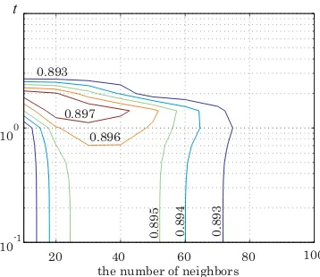
20 40 60 80 100
10-3 10-2 10-1
0.898 0.897
0.896 0.895 0.893
0.894
t
the number of neighbors
Figure 2. Results of the selected dataset byRL
ratings. These results are obtained by the four kernels, CT,RL,NLand DF, which are constructed by changing the number of neighbors ranging fromk= 4tok= 100, as well as the parameter t in (8), (11) and (12), which ranges fromt = 2−10 tot= 210. Note that the contour lines that are less than 0.893 are omitted from Figs. 2 through 4, and those that are less than 0.911 are omitted from Figs. 5 and 6.
From Figs. 1 through 4, we see that the performance of the three kernels, RL, NL and DF, are almost the same and slightly better than that of CT. We can see that the best performance is achieved when the number of neighbors (k) is around 30 for all the kernels. On the other hand, the best results are obtained when the parameter
t is around 10−2 for RL, and t = 1 for NL and DF,
both of which are defined by the normalized Laplacian, ˜
L ≡ D−1/2LD−1/2. It should be emphasized that the proposed method offers fairly high performance in a wide range of parameter settings. Furthermore, Figs. 5 and 6 indicate that almost the same parameter settings generate the highest performance for the case when we use the full dataset.
For comparison, we also perform the same five-fold cross-validation using a previously proposed scoring method by Fouss et al. [3], whose results are listed
0.898
0.897
0.896 0.895
0.894 0.894
20 40 60 80
10-2 10-1 100
t
100 the number of neighbors
Figure 3. Results of the selected dataset byNL
20 40 60 80
10-1 100
0.897 0.896
0.895 0.894 0.893 0.893
100 the number of neighbors
t
Figure 4. Results of the selected dataset byDF
in Table I. We also summarize the highest performance obtained by the four kernels. We can see from this table that, for both selected and full datasets, the three kernels (RL,NLandDF) achieve almost the same performance which are better thanCT, and significantly better than the method by Fousset al.[3] when we use the full dataset.
VI. CONCLUSION
We have introduced new methods for recommendation tasks based on the 1-SVM. Using special structures of graph kernels, we show that the 1-SVM can be formulated as rather simple quadratic programming problems. In addition, the formulations can take advantage of the sparsity of the Laplacian matrix, which results in handling recommendation tasks with over one million ratings. Numerical experiments indicate that the quality of our recommendations is high.
TABLE I.
COMPARISON OF THE BEST DEGREE OF AGREEMENTS
Dataset Fousset al.[3] CT RL NL DF
the number of neighbors
100
20 40 60 80
10-3 10-2
t
0.919 0.9195
0.918 0.9185
0.917 0.916 0.915 0.9140.913
Figure 5. Results of the full dataset byRL
20 40 60 80
t
10-2 10-1 100
0.918
0.917 0.917
0.916
0.916
0.915
0.914
Figure 6. Results of the full dataset byNL
ACKNOWLEDGMENTS
This study was supported in part by Grants-in-Aid for Scientific Research (16201032 and 16510106) from JSPS.
REFERENCES
[1] P. Resnick, N. Iacovou, M. Suchak, P. Bergstorm, and J. Riedl, “GroupLens: An Open Architecture for
Collabo-rative Filtering of Netnews,” inProceedings of ACM 1994
Conference on Computer Supported Cooperative Work. Chapel Hill, North Carolina: ACM, 1994, pp. 175–186. [2] U. Shardanand and P. Maes, “Social information filtering:
Algorithms for automating “word of mouth”,” in
Proceed-ings of ACM CHI’95 Conference on Human Factors in Computing Systems, vol. 1, 1995, pp. 210–217.
[3] F. Fouss, A. Pirotte, and M. Saerens, “A novel way of computing dissimilarities between nodes of a graph, with
application to collaborative filtering,” in 15th European
Conference on Machine Learning (ECML 2004); Proceed-ings of the Workshop on Statistical Approaches for Web Mining (SAWM), 2004, pp. 26–37.
[4] M. Szummer and T. Jaakkola, “Partially labeled
classifica-tion with Markov random walks,” inAdvances in Neural
Information Processing Systems, vol. 14, 2002, pp. 945– 952.
[5] A. Smola and I. Kondor, “Kernels and regularization on
graphs,” in Proceedings of the Annual Conference on
Computational Learning Theory, ser. Lecture Notes in Computer Science, B. Sch¨olkopf and M. Warmuth, Eds. Springer, 2003.
[6] M. Belkin and P. Niyogi, “Semi-supervised learning on
Riemannian manifolds,” Machine Learning, vol. 56, pp.
209–239, 2004.
[7] T. Ito, M. Shimbo, T. Kudo, and Y. Matsumoto,
“Applica-tion of kernels to link analysis,” inKDD ’05: Proceeding
of the eleventh ACM SIGKDD international conference on Knowledge discovery in data mining. New York, NY, USA: ACM Press, 2005, pp. 586–592.
[8] B. Sch¨olkopf, J. C. Platt, J. Shawe-Taylor, A. J. Smola, and R. C. Williamson, “Estimating the support of a
high-dimensional distribution,” Neural Computation, vol. 13,
pp. 1443–1471, 2001.
[9] J. Shawe-Taylor and N. Cristianini, Kernel Methods for
Pattern Analysis. Cambridge: Cambridge University Press, 2004.
[10] F. R. Chung,Spectral Graph Theory. American
Mathe-matical Society, 1997.
[11] X. Zhu, J. Lafferty, and Z. Ghahramani, “Semi-supervised learning: From Gaussian fields to Gaussian processes,” Carnegie Mellon University, Technical Report CMU-CS-03-175, 2003.
[12] O. L. Mangasarian and M. V. Solodov, “Nonlinear comple-mentarity as unconstrained and constrained minimization,” Math. Programming, vol. 62, no. 2, Ser. B, pp. 277–297, 1993.
[13] D. Zhou, O. Bousquet, T. N. Lal, J. Weston, and B. Sch¨olkopf, “Learning with local and global
consis-tency,” Advances in Neural Information Processing
Sys-tems, vol. 16, pp. 321–328, 2004.
[14] B. Sarwar, G. Karypis, J. Konstan, and J. Riedl, “Analysis
of recommendation algorithms for e-commerce,” in EC
’00: Proceedings of the 2nd ACM conference on Electronic commerce. New York, NY, USA: ACM Press, 2000, pp. 158–167.
Yasutoshi Yajima was born in Nagano, Japan. He received his Ph.D., MS, and BS degrees in industrial engineering and management from Tokyo Institute of Technology in 1993, 1990 and 1988, respectively.
He is currently an Associate Professor of Industrial Engineer-ing and Management at Tokyo Institute of Technology in 1993. His current research interests include numerical optimization, operations research and data mining.
Prof. Yajima is a member of the Operations Research Society of Japan.