Jivjendra et al. World Journal of Engineering Research and Technology
FULL-ORDER AND REDUCE-ORDER LINEAR SYSTEM WITH
UNKNOWN INPUT IMPLIMENTATION IN MATLAB/SIMULINK
Jivjendra*1 and Deman Kosale2
1
PG Scholar Department of Electrical Engg. and 2Assistant Professor Department of Electrical Engg.,
Sarguja University Ambikapur Chhattisgarh (India) Vishwavidyalaya Engineering College
Lakhanpur C.G. (India).
Article Received on 25/08/2019 Article Revised on 15/09/2019 Article Accepted on 05/10/2019
ABSTRACT
In this paper full Full-Order and Reduced-Order Linear Systems with
Unknown Inputs Implementations are test both full order and reduce
order observer design and examination of the stability of any linear
system. The system stability test by the coordinate system they system
are used provided the all existence condition. The full order observer
are observed in all state and reduce order observer is estimated by the
state reduce order observer are more complex. The advantages of the
reduce observer avoiding the reconstructing accessible states design.
Drawback and advantage the examination technique is pointed andillustrated by the matlab
simulation in numerical examples. The theoretical results have also been developed how to
set up the reduced-order initial conditions using the least-squares method, derived and an
observation that the reduced-order observer output is identical to the original system’s actual
output, the result established by matlab/simulink model.
KEYWORDS: Matlab simulation, full order observer, reduce order observer, unknown input, linear system.
1. INTRODUCTION
The proposed system are Hopefully by understanding full- and reduced-order observer design
and Matlab/Simulink implementation, students, instructors, engineers, and scientists will
World Journal of Engineering Research and Technology
WJERT
www.wjert.org
SJIF Impact Factor: 5.924*Corresponding Author
Jivjendra
appreciate the importance of observers and feel confident using observers and observer-based
controllers in numerous engineering and scientific applications. In the control systems, time
invariant linear systems are represented, in state-space form, by,
=Ax(t)+Bu(t), x (0) = x0 (1)
Where x(t) is the state-space vector of dimension n, u (t) is the system input vector (which
may be used as a sys-tem control input) of dimension m, and matrices A and B are constant
and of appropriate dimensions. In practice, the initial condition is often unknown, in which
case an observer is designed. estimate or observe system state-space variables at all times.
To take the advantage of the useful features of feedback (see, for example, it is often assumed
that all state variables are available for feedback (full-state feedback), allowing that a
feedback control input can be applied as,
u(x(t))=-Fx(t), (2)
Where F is a constant feedback matrix of dimension m # n. The fact that all state-space
variables must be available for feed-back is a prevalent implementation difficulty of full-state
feedback controllers. Moreover, large-scale systems with full-state feedback have many
feedback loops, which might become very costly and/or impractical. Moreover, often not all
state variables are available for feedback. Instead, an output signal that represents a linear
combination of the state-space variables is available,
y (t)= Cx(t) (3)
Where dim " y (t), = l < n = dim "x (t),. It is assumed that
l = c = rank=C, so there are no redundant measurements. In such a case, under certain
conditions, an observer can be designed that is a dynamic system driven by the system input
and output signals with the goal of reconstructing (observing, estimating) all system
state-space variables at all times.
This article shows how to implement full- and reduced-order observers using the Matlab and
Simulink software packages for computer-aided control system design. In fact, how to
implement a linear system and its observer, represented by their state-space forms, using the
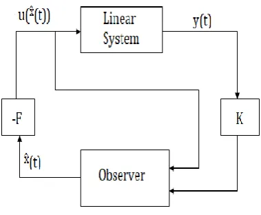
Fig. 1: A block diagram for the system observer configuration.
2. FULL-ORDER OBSERVER DESIGN
The theory of observers originated in the mid 1960s According to any system driven by the
output of the given system can serve as an observer for that system. Consider a linear
dynamic system,
(t) =Ax(t) + Bu(t), x(t0)= x0 = unknown,
y(t) = Cx(t). (4)
The system output variables y(t) are available at all times, and that information can be used to
construct an artificial dynamic system of the same order nth as the system under consideration that can estimate the system state-space variables at all times. Since the matrices A, B, C are
known, it is rational to postulate an observer for (4) as,
(t) = A (t ) +Bu (t),
(t0)= 0, (5)
If the outputs y (t) and y (t) are compared, they will, in general, be different since, in the first
case, the initial condition of (4) is unknown, and, in the second case, the initial condition of
the proposed observer (5) is chosen arbitrarily by a control engineer (designed). The
difference between these two outputs generates an error signal,
Which can be used as the feedback signal to the observer such that the estimation
(observation) error e (t) = x (t) -xt (t) is reduced. An observer that takes into account feedback
information about the observation error,
(t) = A (t ) +Bu (t) + K (y(t) - (t))
A (t ) +Bu (t) + KCe (t), (7)
Where the matrix K represents the observer gain, which must be selected such that the
observation error tends to zero as time increases. From (4) and (7), comes an expression for
dynamics of the observation error,
(t) = (A - KC)+ e(t), e ( t0) = unknown. (8)
If the observer gain K is chosen such that the feedback matrix A KC is asymptotically stable
(has all eigenvalues with negative real parts), then the estimation error e (t) will decay to zero
for any initial condition e (t0). This stabilization requirement can be achieved if the pair (A,
C) is observable. It can be also noted that the error (and observer) stabilization can be
achieved under a weaker condition that the pair (A, C) is detectable (not all, but at least the
unstable modes of matrix A are observable).
A standard rule of thumb is that an observer should be designed such that its response is
much faster than the sys-tem. This is especially important when the observed state variables
are used for the purpose of feedback control. This can be achieved theoretically by choosing
the observer eigenvalues to be about ten times faster than the system eigenvalues. that is by
setting the smallest real part of the observer eigenvalues to be ten times larger than the largest
real part of the closed-loop system eigenvalues.
Since the system changes in time, its estimated state variables must be as current as possible,
otherwise the feedback signals represent considerably delayed estimates of the actual state
variables, which can make the controller inaccurate and inefficient. │Re{λmin(A-KC)}│observer>10
Re{λmmax(A-BF)}│system (9)
Theoretically, an observer can be made arbitrarily fast by locating its closed-loop eigenvalues
very far to the left in the complex plane, but very fast observers can generate noise, which is
After the system eigenvalues λi (A -BF) are deter-mined, the observer eigenvalues λi (A -
KC) are placed in the desired locations by selecting the corresponding ob-server gain K using
the eigenvalue assignment technique.
2.1 Separation Principle
It is important to point out that the system-observer con-figuration preserves the closed-loop
system eigenvalues that would have been obtained if the linear, perfect-state-feedback control
had been used. This fact is shown below.
The system (4) under perfect state-feedback control, that is, u(x(t)) Fx(t) has the closed-loop
form,
(t) = (A - BF)x(t), (10)
So that the eigenvalues of the matrix A - BF are the closed-loop system eigenvalues under
perfect state feedback. In the case of the system-observer configuration, the actual control
signal applied to both the system and the observer is
u( (t)) = -F (t) = -Fx(t) + Fe(t) (11)
From (8), (10), and (11),
= =A
Since the state matrix of this augmented system is upper block triangular, its eigenvalues are
equal to the union of the eigenvalues of the matrices A - BF and A -KC. A very simple
relation among x( t), e (t), and x ( t) can be written using the definition of the estimation error
as
= = T
Note that the matrix T is nonsingular. To go from xe-coordinates to x -coordinates.
3. Full-Order Observer Implementation in Simulink
An observer, being an artificial dynamic system of the same order as the original system, can
be built by a control engineer using either capacitors and resistors (what electrical engineers
do) or using masses, springs, and frictional elements or simply using a simulink modal that
anybody with a basic knowledge of control systems and differential equations can do,
especially those familiar with Matlab and Simulink.
(t) = A (t) + Bu(t) + K(y(t) – (t))
(t) = c (t) (12)
In practice, the observer is implemented as a linear dynamic system driven by the original
system input and output signals, that is, u (t) and y(t). Eliminating y (t) from the observer
equation (12) yields the observer form used in practical implementations,
(t)=(A-KC) (t)+Bu(t)+ Ky(t). (13)
The corresponding block diagram of the system-observer configuration, also known as the
observer-based controller configuration, is presented in Figure with the feedback loop closed
using the feedback controller as defined in namely u( (t )) = -F (t).
The state-space block of Simulink is used. That block allows only one input vector and one
output vector. For that reason, the observer is represented as a system with one augmented
unknown input,
=(A-KC) (t)+[BK] (14)
Using the given dimensions of the state, input, and output variables (respectively n, m, and c),
the system matrices for the state-space Simulink blocks are set as follows. For the system, the
matrices are respectively: A, B, C, zeros(c,m), the last one meaning a zero matrix of
dimensions cm.
The results obtained for y(t) and (t) and output observation error e(t) may be presented
using the Simulink block “scope,” or passed to the Matlab window, together with time, where
they can be plotted using the Matlab plot function. For example, plot(t,error) plots the output
observation error as a function of time. t Such a plot (or figure) can be further edited using
numerous Matlab figure-editing functions. For the observer, the corresponding matrices
should be set using information from,
Observer State Space
Block Setup
A – K * C, [B K], eye(n),
The first matrix is the observer feedback matrix, the second is the augmented matrix of two
inputs into the observer and the third matrix (set to the identity of n dimension) indicates that
estimates of all n state variables are available on the observer output. Since the observer is a
system either built by a designer or a computer program that simulates observer dynamics,
the designer has full freedom to choose the observer output matrix and set it to an identity
matrix so that all observed (estimated) state space variables appear on the observer output.
The fourth matrix represents the matrix “D” in the observer block and, due to the fact that the
input matrix into the observer is the augmented matrix [B K] of dimension n*(m+c) and the
output matrix from the observer is of dimension n*n (identity matrix In), the dimension of the
zero matrix must be n*(m+c) Finally, the last entry in denotes the observer initial condition
vector that can be set arbitrarily. Later on in the article, a rational choice of the observer
initial condition will be discussed. These matrices can be entered in the Simulink state-space
block by double left clicking on the observer state-space block, which will open a new window as shown in Figure For details, see “Matlab Code: System State-Space Block Setup.”
4. REDUCE-ORDER OBSERVER DESIGN
Consider the linear dynamic system defined with the corresponding measurements. Assume
that the output matrix C has full rank (equal to c) so that there are no redundant
measurements. This means that the output equation y(t)= Cx(t) represents, at any time, c
linearly independent algebraic equations for n unknown state variables x(t). Note that y(t), of
dimension, c is the measured system output, and hence is known at all times. In this section,
it is shown how to construct an observer of reduced order r = n - c for estimating the
remaining r state-space variables [c state variables can be obtained directly from the system
measurements y(t)= Cx(t)]. As indicated the reduced-order observer should be used when the
system measurements have no noise. If noise is present, it is better to use the full-order
observer, since it filters the system measurements and, in general, all state variables.
It will be seen that the procedure for obtaining the reduced-order observer is not unique. An
arbitrary matrix C1 of dimension r*n whose rank is equal to r = n - c can be found such that
the augmented matrix,
rank = n,
has full rank equal to . n Introduce a vector p(t) of dimension r such that
x(t),
which can be solved to obtain
(t)=Ly(t)+L1 (t)
Where y(t) are known system measurements and (t) has to be obtained using a
reduced-order observer of dimension. r<n As a preliminary result in the process of constructing a
reduced-order observer for p(t) it can be noticed from that the following algebraic relations
exist,
In = [L L1] = = (16)
giving CL= IC, CL LI = Ir, CL1=0, C1L=0, where In, Ic, Ir are identity matrices of corresponding dimensions and n=c+r.
Since from p(t) = C1x(t) the differential equation for p(t) can be easily constructed using the original system differential equation which leads to,
= (p(t)) = (c1x(t)) = C1 (t)
= C1Ax(t)+C1Bu(t)
= C1AL1p(t)+C1Bu(t) (17)
To design an observer for p(t) using the above established principal
Y(t) = Cx(t) =CLy(t) + CL1p(t) = y(t)+0 =y(t) (18)
More information about y(t) can be obtained from the knowledge of (t), in which case
(t) = C (t) = CAx(t)+CBu(t)
= CAL1p(t)+CALy(t)+CBu(t). (19)
This indicates that (t) contains information about p(t), so that it can be used to construct an
observer for p(t)
(t)=C1AL1 (t)+C1ALy(t)+C1Bu(t)+ K1( (t)- (t)), (20)
Where K1 is the reduced-order observer gain, which has to be determined such that the
observer measurement is obtained from by replacing. p(t) by its estimate (observation) (t),
that is,
(t)=CAL1 (t)+CALy(t)+CBu(t). (21)
Signal differentiation is not a recommended operation since it is very sensitive to noise;
signal differentiation amplifies noise so it should be avoided in all practical applications.
Using an appropriate change of variables, it is possible to completely eliminate the need for
information about the derivative of the system measurements (t).
4.1 Setting Reduced-Order-Observer Eigenvalues in the Desired Locations
As discussed in good performance typically requires placing the reduced-order observer
eigen values such that the reduced-order observer is roughly ten times faster than the system whose speed is determined by the closed loop system eigen values given by λ(A-BF) Note
that the reduced-order observer matrix can be written as,
Aq=C1AL1-K1CAL1=(C1AL1) – K1(CAL1)
To determine the order observer gain K1 such that it arbitrarily places the
reduced-order observer eigen values, the pair (C1AL1,CAL1) must be observable. The next subsection will show that this condition is satisfied if the original system is observable (the pair (A,C) is observable). See “Reduced-Order-Observer Design Process” for details on the steps involved
in the design of this observer.
4.2 Reduced-Order Observer Design with a Change of State Coordinates
It is shown first in this subsection that a reduced-order observer can be also designed with a
change of state coordinates. More importantly, with this change of state coordinates, it
becomes easy to prove the result that if the original system is observable then the
reduced-order observer is also observable.
Consider a linear system with the corresponding measurements defined in (4). The
reduced-order observer design can be simplified, and some important conclusions can easily be made
using a nonsingular transformation pn*n
Such that
Y(t) = Cx(t) = CP-1Px(t) = CP-1
= [Ic 0] = x1(t) (22)
To map the system into new coordinates in which the system measurements provide complete
information about a part of the state-space vector x1(t) of dimension. c In such a case, an observer is needed to estimate the remaining part of the state-space vector, that is, x2(t) of dimension r = n-c. This is possible since there exists a transformation P of the full-rank
matrix, C obtained using elementary transformations, such that CP-1 = [Ic 0]. This procedure can be found in many standard linear algebra. Such a transformation is defined in so that.
CP-1 = C[ L L1] = [CL CL1] = [I 0]
5. Extension to Kalman Filtering
By mastering the design of deterministic observers presented in this article, more complex
linear dynamic estimation problems can also be considered, for example, the Kalman filtering
and other optimal linear estimation problem In fact, the Kalman filter can also be
implemented as a software program in Matlab/Simulink using the methodology presented in
this article. For a linear dynamic system disturbed by a Gaussian white noise stochastic
process w(t) and system measurements corrupted by a Gaussian white noise stochastic
process v(t)
(t) = AX(t) + Bu(t) + Gw(t),
Y(t) = Cx(t) + v(t) (23)
The kalman filter is given by
KF (t) = (A-KC) KF (t) + Bu(t) + KKFy(t), (24)
Which is exactly the same structure as the full-order observer structure is presented. The
6. Full And Reduce Order Observer Designs For An Aircraft Model 6696 . 0 1 . 9 0 00057 . 0 1 214 . 1 0 0001212 . 0 0 214 . 1 0 00012 . 0 0 3 . 46 2 . 32 01357 . 0 A 1577 . 0 1394 . 0 1394 . 0 433 . 0 B 0 0 0 1 1 0 0 0 C 0 0 D
Matrix C1 needed for the reduce-order observer design is chosen
0 1 0 0 0 0 1 0 1 C
See “Matlab Program for the Aircraft Simulation Example” for the corresponding Matlab
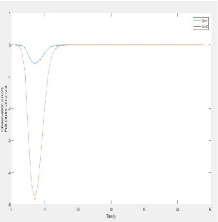
program with all simulation data. The obtained differences between the actual and estimated
state trajectories using the full- and reduced-order observers are presented in Figure 2 and 3.
In both cases, the initial conditions for the observers are obtained using the least-squares
formulas. It can be seen from Figures 4 to 7 that the reduced-order observer performs better
than the full-order observer. Not only are there no observation errors for the two state
variables directly measured, but the reduced-order observer is also more accurate than the
full-order observer. Note that the eigenvalues for both observers are placed to be of the same
speed.
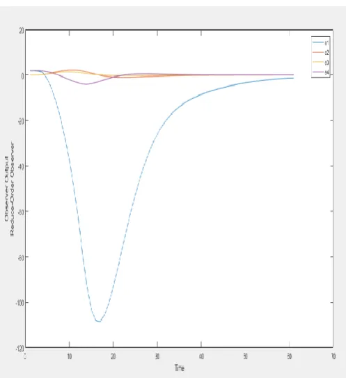
The reduced-order observer eigenvalues are placed at -10, -11 and the full-order observer
eigenvalues are placed at -10, -11, -12, -13. Moreover, the reduced-order observer is simpler
for implementation, since it is a dynamic system of lower order than the original system. An
additional advantage of the reduced-order observer is that they require fewer sensors and
fewer feedback loops for corresponding feedback control applications.
The importance of Matlab/Simulink implementation of the full- and reduced-order observers
has been demonstrated in the previous sections of this article. These results can be used in all
7. SIMULATION AND RESULT
The Full-Order and Reduce-Order observer is obtained by matlab simulink the system is
work on the pole placement method it is find the system stability. On the system stable then
method is not work but the system are unstable then the find unstable pole location and pole
is place by desired location in required characteristic equation on the system the simulink
Fig. 4: System error.
Fig. 6: Full-order Output.
Fig. 7: Reduce-order Output.
8. CONCLUSION
In this proposed system has been shown in detail how to implement Full-order and
Reduce-order observer in matlab/simulink. The fundamental method are conclude by the system
The stability are find in the drown in the figure by given characteristic equation to check the
stability of any system. In this method are implement by the required input and output are
increase then the system are use in the more input and also more output in future work.
The system are use in the closed loop system it main work to get required output in the
system. The system are more useful in the find system stability it is very easy to implement in
the personal and industrial uses to change the system input and output.
REFERENCES
1. O. Boubaker, B. Sfaihi, “Robust observers for linear systems with unknown inputs: A comparative study,” to appear in IEEE SSD’2005, Sousse, Tunisia, 2005.
2. N. Nise, Control Systems Engineering. Hoboken, NJ: Wiley, 2008.
3. S. P. Bhattacharyya, “Observer design for linear system with unknown inputs,” IEEE
Trans. Automat. Contr., 1978; AC-23: 483-484.
4. K. Ogata, Modern Control Engineering, 3rd edition, Prentice Hall, New Jersey, 1997. 5. M. Darouach, M. Zasadzinski, and S. J. Xu, “Full-Order observers for linear systems with
unknown inputs,” IEEE Trans. Automat. Contr., 1994; AC-39: 606-609.
6. Chang, S. K., W. You, and P. L. Hsu (1994), General-Structured Unknown Input
Observers, Proceedings of the American Control Conference Baltimore, Maryland,