INTRODUCTION
Urban areas modify the atmospheric envi-ronment, for instance through the changes of the city’s thermal conditions as a result of progressive development and loss of vegetation [Nikolopou-lou and Lykoudis 2006, Boumans et al. 2014, van Hove 2015], and changes to air chemistry through the presence of particulate and gas pollution, which includes tropospheric ozone [Carnero et al. 2010]. The tests carried out in Seattle showed an approx. 10% increase in A&E visits caused by asthma attacks along with increased levels of O3 by each 10 ppb [Goodin, Hubbard 2016]. Addi-tionally, among the children aged 6–15, O3 and PM2.5 particulate lead to a decrease in the lung capacity [Chen et al. 2015]. Novack et al. [2016] showed the impact of air pollution on the oxida-tive stress of a human body. In their tests, they noted an inverse relation between the high
con-centration of O3 and a positive relation between suspended particulate PM10 and multiplication of blood stem cells. The impact of tropospheric ozone concentration on the respiratory system is confirmed by numerous studies from all over the world: Kinney et al. [1996], Frischer [1999], O’Lenick et al. [2007], Khatri et al. [2001], Tager et al. [2003], Uysal and Schapira [2005]. The re-search also shows an increase in the death rate by 2% due to hypofunction of the cardiovascular system caused by O3 pollution on each 10µg·m-3 [Khaniabadi, et al. 2017]. Tropospheric ozone is a secondary pollutant that arises from a series of photochemical reactions [Clapp and Jenkin 2001,Kleinman 2005, Monks et al. 2015, Tiwari et al. 2015]. Moreover, the solar radiation neces-sary to start the chain reaction, which includes: NOX (NO + NO2), CO, VOC’s and NMVOCs, is absorbed by the human body. The absorption depends on the factors such as: the intensity and
Published: 2018.07.01
Volume 19, Issue 4, July 2018, pages 207–216
https://doi.org/10.12911/22998993/89782
Assessment of Ground Ozone Level under The Physiological
Strain Conditions
Robert Krzysztof Sobolewski
1, Robert Kalbarczyk
11 Wrocław University of Environmental and Life Sciences, Institute of Landscape Architecture, Grunwaldzka 55,
50-357 Wrocław, Poland
* Corresponding author’s e-mail: [email protected]
ABSTRACT
Urban areas are characterised by the impact of negative environmental factors, such as: stress connected with ex-treme bio-thermal conditions or the presence of high concentrations of air pollutants. This study aims to evaluate the relationship between the hours of O3 concentrations and the levels of physiological strain (PhS) in Legnica, during the period from December 2013 to November 2014. The hourly concentrations of O3, NO2 and meteorologi-cal elements used in the study were obtained from the State Environmental Monitoring station in Legnica (Lower Silesia). The evaluation of the bio-thermal conditions was carried out by means of the physiological strain indica-tor (PhS). The basic statistics were subject to analysis, the frequency of hourly pollution concentrations and the
thermal strain were evaluated, as was the Pearson correlation coefficient and multiple regression between O3 and
PhS. A detailed analysis was carried out for the summer months (June-August). The most adverse conditions in terms of pollution with tropospheric ozone and heat strain were noted in July. The strongest relations between O3
and PhS were observed in June. In winter months (December-February) no significant dependencies were noted
between the tested variables. These tests will help to contribute to increasing the current knowledge on evaluating the thermal comfort of urbanised areas and the accompanying aero-sanitary conditions.
structure of solar radiation, the Sun’s altitude (h), ground albedo, body-to-sun orientation and the insulating power and colour of clothing and skin [Błażejczyk 2004]. The highest concentration of O3 occurs at noon, showing an inverse meridian course from NO2, NO and NOx [Escudero et al. 2004, Kalbarczyk et al. 2015, Rozbicka and Roz-bicki 2016, Zheng et al. 2017]. In the same hours, the least favourable bio-thermal conditions are observed that impact the human body [Park et al. 2014, Kalbarczyk et al. 2015]. High O3 concen-tration is often accompanied by a high air tem-perature [Vandentorren et al. 2004, Pascal et al. 2012]. Błażejczyk and McGregor [2007], on the basis of 3 bio-thermal indicators: STI, PST, PhS, showed that in London it is possible to explain 20–29% deaths by the certain values of these in-dicators occuring three days earlier. In Poland, according to Błażejczyka and others [2017], one may expect an increase in mortality on the days characterized by strong and very high heat con-centration, with reference to the days when heat stress is observed, by 12% and 47% respectively.
The aim of the study was to evaluate the re-lationship between the hours of O3 concentrations and the levels of physiological strain (PhS) in Legnica, during the period from December 2013 to November 2014.
MATERIALS AND METHODS
Legnica is located in the west of Poland, in the Lower Silesia region (51°12′36″N, 16°09′42″E, hs = 113–168 m. a.s.l.). It is the eighth largest (56 km2) and densely populated (1802 people·km-2) city in the region and the third largest in terms of population (100886 people) af-ter Wrocław and Wałbrzych [Central Statistical Office 2015]. Legnica belongs to the central bio-climatic region of weak stimulusity, characterised by an average air temperature at 12:00 (UTC) of 21.3°C in the summer and 1.9°C in the winter [Błażejczyk and Matzarakis 2007]. This study uses the data of hourly pollution concentrations of O3, NO2 and the meteorological data during the period from December 2013 to November 2014. The data was obtained from the State Environ-mental Monitoring Station in Legnica, marked by the international code PL0190A, indicating a city type station. The data was prepared for universal time (UTC). The initial data verification was car -ried out on the basis of the correlation between
the O3 hourly concentration and total radiation (Rad, W∙m-3), air temperature (Ta, °C), relative air humidity (Rh, %), as well as the wind speed (v, m·s-1) analysis which showed occurrence of two separate data sets. The daily distribution of average values of the meteorological elements showed a sudden drop in the total radiation val-ues between 12:00 and 14:00, depending on the particular month analysed within the researched period, probably caused by the shadowing of the station in the afternoon. The basis of the division into two data sets was the result of carrying out a distribution of average hourly values of meteoro-logical elements for individual decades of each month. The data sets obtained in this way were further used in the correlation analysis.
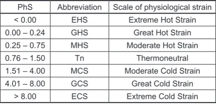
The evaluation of pollution with the concen-trations of O3 and NO2 in particular months of the research period was carried out on the basis of descriptive statistics and an analysis of hourly concentration frequencies of O3 and NO2 in the adopted classes of pollution levels, consecutively for ozone: 0–40, 41–80, 81–120, >120 µg·m-3 and for nitrogen dioxide: 0–20, 21–40, 41–60, 61–80, >80 µg·m-3. The evaluation of the bio-thermal con-ditions was carried out on the basis of the physi-ological strain (PhS, dimensionless) (Table 1).
The PhS indicator values were calculated by means of the Bioklima 2.6 software (https://www. igipz.pan.pl/Bioklima-zgik.html). The PhS indi-cator is expressed as the relation of heat loss from a human body by convection (C) to its loss as a re-sult of perspiration evaporation (E) [Błażejczyk, Matzarakis 2007]:
(1) For each month, there is a frequency related to the occurrence of different concentrations of physiological strain. In turn, the occurrence fre-quencies of the adopted O3 concentration in par-ticular classes of physiological strain
concentra-Table 1. Scale of physiological strain (PhS)
PhS Abbreviation Scale of physiological strain < 0.00 EHS Extreme Hot Strain 0.00 – 0.24 GHS Great Hot Strain 0.25 – 0.75 MHS Moderate Hot Strain
0.76 – 1.50 Tn Thermoneutral
1.51 – 4.00 MCS Moderate Cold Strain 4.01 – 8.00 GCS Great Cold Strain
tion were evaluated only for the chosen months characterised by a large and moderate hot strain. For the month of the most frequent extreme con-ditions in the O3 concentrations above 120 µg·m-3 and hot strain load, an analysis of the daily distri-bution of O3, NO2, values PhS concentration and meteorological elements in subsequent decades was conducted. Due to the asymmetric, right-hand character of the hourly NO2 concentration schedule, this data was adapted to a normal sched-ule. In order to do so, the hourly data was stated as a logarithm, which enabled carrying out fur-ther statistical analyses. An analysis of the Pear-son correlation coefficient between the O3 and meteorological elements and PhS indicators was carried out for three groups: including the full set of all-day measurements data, morning measure-ments, that is from sunrise to 13:00 and afternoon measurements data – from 14:00 to sunset. The correlation was evaluated on the level of p=0.05. For the months when the correlation analysis was statistically significant, the equations of multiple regression analyses between tropospheric ozone and conditions of physiological strain in the pres-ence of NO2 were built.
RESULTS
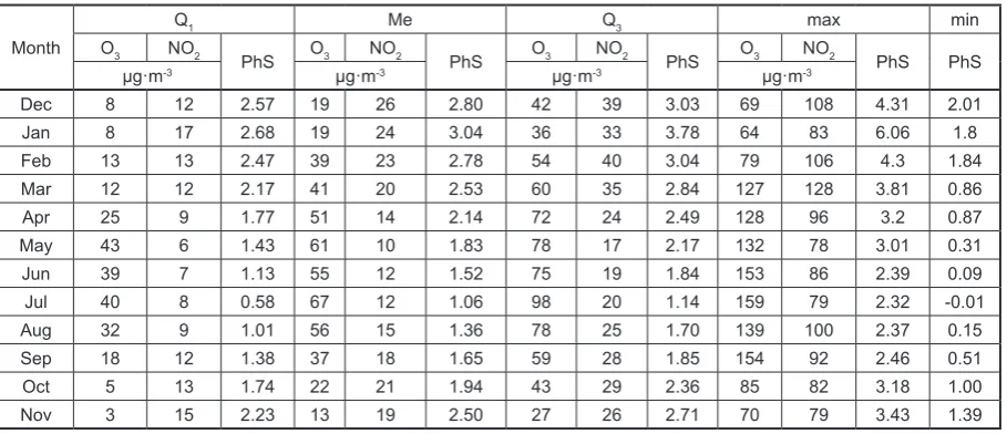
The descriptive statistics showed that from March to September, the maximum hourly O3 concentration values in particular months exceed-ed 127 µg·m-3 (Tab. 2)
. The highest concentration was recorded in July at 159 µg·m-3. In turn, the highest NO2 concentration in the summer period fell in August and was 100 µg·m-3. In the same
month, the median value calculated for the NO2 emission was equal to 15 µg·m-3
. In the month when the highest O3 concentration was docu-mented, the value of the PhS indicator amounted to -0.01, which indicates the occurrence of “ex-treme hot strain” conditions. In the remaining summer months, i.e. June and August, the maxi-mum values of the PhS indicator showed the con-ditions of “great hot strain”. In the winter months (December-February) the maximum monthly O3 concentration did not exceed 70 µg·m-3, the high-est recorded in January – 69 µg·m-3
. In the same month, the maximum value of the PhS indicator amounted to 6.06. This confirms the occurrence of “great cold strain” in this month. The maxi-mum concentration of NO2 was documented in March at 128 µg·m-3;moreover, the maximum concentration above 100 µg·m-3 was also re-corded in December and February. The value of the third percentile indicates that in July, 25% of all O3 concentrations were over 98 µg·m-3; in comparison, in January, 25% of all concentra-tions were within the range of 36–64 µg·m-3
. The highest median values above 50 µg·m-3occurred in July, May, August, June, and April. Thus, the median value for the spring-summer months was higher than the value of the third percentile for winter months.
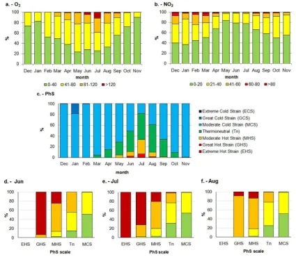
In July, around 40% of all cases constituted the hourly concentrations above 80 µg·m-3; out of that concentration >120 µg·m-3 amounted to approx. 11.5% (Fig. 1). March was characterised by the least favourable conditions in terms of the frequencies hourly concentrations of NO2; the concentrations above 80 µg·m-3 constituted 2.8% of recorded cases, in turn, in the scope of 60–80
Table 2.Descriptive statistics for individual months of the research period: Dec. 2013 – Nov. 2014
Month
Q1 Me Q3 max min
O3 NO2
PhS O3 NO2 PhS O3 NO2 PhS O3 NO2 PhS PhS
µg·m-3 µg·m-3 µg·m-3 µg·m-3
Dec 8 12 2.57 19 26 2.80 42 39 3.03 69 108 4.31 2.01
Jan 8 17 2.68 19 24 3.04 36 33 3.78 64 83 6.06 1.8
Feb 13 13 2.47 39 23 2.78 54 40 3.04 79 106 4.3 1.84
Mar 12 12 2.17 41 20 2.53 60 35 2.84 127 128 3.81 0.86
Apr 25 9 1.77 51 14 2.14 72 24 2.49 128 96 3.2 0.87
May 43 6 1.43 61 10 1.83 78 17 2.17 132 78 3.01 0.31
Jun 39 7 1.13 55 12 1.52 75 19 1.84 153 86 2.39 0.09
Jul 40 8 0.58 67 12 1.06 98 20 1.14 159 79 2.32 -0.01
Aug 32 9 1.01 56 15 1.36 78 25 1.70 139 100 2.37 0.15
Sep 18 12 1.38 37 18 1.65 59 28 1.85 154 92 2.46 0.51
Oct 5 13 1.74 22 21 1.94 43 29 2.36 85 82 3.18 1.00
µg·m-3 – 4.2%. In July 2014, the conditions con-nected with hot strain constituted 30% cases. In June and August, the frequencies were compa-rable, amounting to approx. 11% and 9.7%. In the winter period (December-February), there were almost the same conditions connected with “mod-erate cold strain”, except for January when 18.4% of cases were characterised by “great cold strain”. In the remaining months, the strain did not ex-ceed 1%. In the researched period, there were no extreme thermal strain days. Only in July was there a single case of “extreme hot strain”. The occurrence of “moderate hot strain” in September was 1.4%, in May approx. 4.5%. The summer pe-riod, from June to July, was characterised by the occurrence of thermal conditions from “moder-ate cold strain” to “extreme hot strain”. In July and in June the frequency of O3 concentrations above 120 µg·m-3 was connected with the condi-tions of hot strain. Extreme condicondi-tions were
re-corded only in July, which constituted an isolated case. In June, during the “moderate hot strain” approx. 93% cases involved the concentrations above 120 µg·m-3. In turn, August was character-ised by, in comparison to the remaining summer months, a lower frequency of O3 concentrations above 120 µg·m-3.
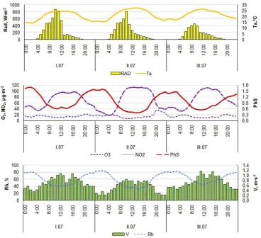
The average hourly O3 exceeded the value of 100 µg·m-3 in the second and third decades of July, from 10:00 to 18:00 and from 11:00 to 17:00 (Fig. 2). NO2 does not show a high change-ability of average daily concentration in partic-ular decades. The highest concentration in the second decade was recorded at night. The daily distribution of average O3 concentrations shows a reverse distribution in reference to the PhS val-ues. The lower values of PhS indicator show the occurrence of the hot strain in the second decade, where the least favourable PhS conditions are re-corded, which overlaps with the high level of O3
Fig. 1. Occurrence frequencies: the hourly concentrations of gas pollution O3 and NO2 (a – b), thermal strain in
concentrations. The solar radiation values show a clear, untypical, drop in the afternoon, which is probably caused by the shadowing of the moni-toring station. In the third decade, we can notice a slight increase of the air temperature during the night, which may indicate the effect of the urban heat island present in the research period. The increase of the temperature is accompanied by a slight increase of the tropospheric ozone and the drop in the PhS indicator value.
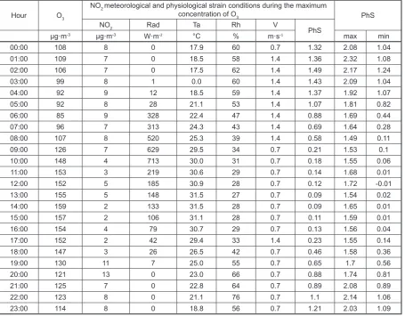
The maximum hourly O3 concentrations in July above 150 µg·m-3 were recorded between 11:00 and 17:00; they were accompanied by low NO2 concentrations in the range from 2 to 5 µg·m-3 (Tab. 3). From 9:00 to 17:00, the highest hourly O3 concentrations occurred during signifi -cant moderate and great hot strain. Such condi-tions were favoured by: low relative air humid-ity below 34%, air temperature above 29°C, and relatively low wind speed approx. 0.7 m∙s-1. Only between 8:00 and 10:00, the maximum O3 con-centration was accompanied by solar radiation in the range of 520–713 W∙m-2. At 11:00 total
radia-tion accompanying maximum O3 values amount-ed to 219 W∙m-2 and gradually decreased in the following hours. The maximum O3 concentration amounting to 159 µg·m-3 was recorded at 14:00 with the PhS value of 0.09. The least favourable thermal conditions connected with very strong hot strain occurred at 12:00 during the maximum O3 concentration, amounting to 152 µg·m-3.
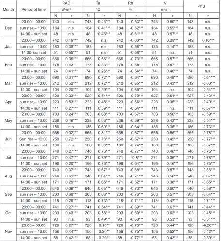
In the winter period, there was no significant correlation between the hourly O3 concentra-tions and the values of the PhS indicator (Tab. 4) A weak correlation (r=0.16, p=0.01) for the data set from 24 h in January constituted an exception. This proven relation has a positive direction, in contrast to the proven relations in the remain-ing months, which adopted a negative direction (March-November). The reason for the change in the direction of relations between the O3 concen-trations and the PhS values in January could be a lack of correlation between O3 and Ta for all pos-sible data sets. The strongest, negative relation (r = -0.87, p=0.01) was recorded in June for the afternoon data set, between 14:00 and 19:00, that
Fig. 2.Daily distribution of average hourly values: O3, NO2, PhS and meteorological elements: total radiation
Rad, (W·m-2) air temperature (Ta, ºC), relative air humidity (Rh, %), wind speed (V, m·s-1) in individual decades
is sunset. For the data from 24 h, the strongest negative correlations in June and July, were r = -0.78 (p=0.01) and r = -0.76 (p=0.01), respective -ly. In the spring period (March-June) and in Sep-tember, clear differences in the relations between the morning data sets – from sunrise to 13:00 and in the afternoon – from 14:00 to sunset, were observed. In July and August, the strength of the correlation between O3 and PhS was comparable both for data from 24 h and from morning and af-ternoon data sets. In June in the afaf-ternoon hours, the strongest correlation between O3 and Ta (r = 0.90, p=0.01) was observed. The relation between the hourly O3 concentrations and total radiation for the data set of afternoon measurements in May and June did not show statistical relevancy on the level of p=0.05.
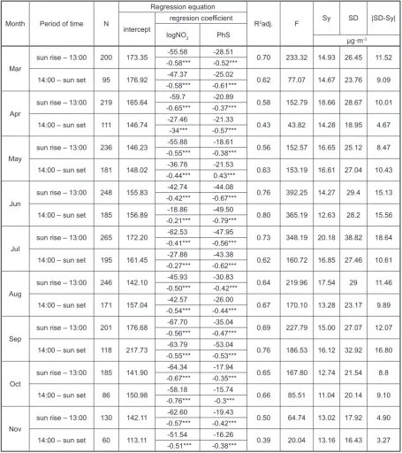
The model of rolling multiple regression was prepared for the months in which there was a significant correlation between O3 and PhS (Table 5). When examining the model, apart from the PhS indicator, additional hourly NO2 values in the form of the common logarithm
were taken into account. In the adopted models, significant impact of all changeables explain -ing the size of O3 immision was confirmed. The greatest fit of the empirical data to the regression function, amounting to 76% and 80%, was ob-tained for June, for the conditions in the morn-ing and afternoon; in turn, the smallest fit was observed in April (58%, 43%) and in November (50%, 39%). On the basis of the partial correla-tion factor, stronger conneccorrela-tions between O3 and bio-thermal conditions, other than NO2 pollu-tions were proven in the afternoon hours. In the morning hours, a greater impact of NO2 on O3 was recorded, in the prepared model.
DISCUSSION
The research carried out between December 2013 and November 2014 showed a significant relationship between the level of tropospheric ozone and unfavourable bio-thermal conditions connected with hot strain. These relations are
Table 3.Maximum O3 concentration at particular hours of July 2014 in reference to the accompanying
meteoro-logical and bio-thermal conditions
Hour O3
NO2 meteorological and physiological strain conditions during the maximum
concentration of O3 PhS
NO2 Rad Ta Rh V
PhS
µg·m-3 µg·m-3 W·m-2 °C % m·s-1 max min
00:00 108 8 0 17.9 60 0.7 1.32 2.08 1.04
01:00 109 7 0 18.5 58 1.4 1.36 2.32 1.08
02:00 106 7 0 17.5 62 1.4 1.49 2.17 1.24
03:00 99 8 1 0.0 60 1.4 1.43 2.09 1.04
04:00 92 9 12 18.5 59 1.4 1.37 1.92 1.07
05:00 92 8 28 21.1 53 1.4 1.07 1.81 0.82
06:00 85 9 328 22.4 47 1.4 0.88 1.69 0.44
07:00 96 7 313 24.3 43 1.4 0.69 1.64 0.28
08:00 107 8 520 25.3 39 1.4 0.58 1.49 0.11
09:00 126 7 629 29.5 34 0.7 0.21 1.53 0.1
10:00 148 4 713 30.0 31 0.7 0.18 1.55 0.06
11:00 153 3 219 30.6 29 0.7 0.14 1.68 0.01
12:00 152 5 185 30.9 28 0.7 0.12 1.72 -0.01
13:00 155 5 148 31.5 27 0.7 0.09 1.54 0.02
14:00 159 2 133 31.5 28 0.7 0.09 1.65 0.01
15:00 157 2 106 31.1 28 0.7 0.11 1.59 0.01
16:00 154 4 79 30.7 29 0.7 0.13 1.56 0.04
17:00 152 2 42 29.4 33 1.4 0.23 1.55 0.14
18:00 147 3 26 26.5 42 0.7 0.46 1.58 0.36
19:00 130 11 7 25.0 55 0.7 0.65 1.7 0.56
20:00 121 13 0 23.0 66 0.7 0.88 1.74 0.81
21:00 125 7 0 22.8 64 0.7 0.89 2.08 0.89
22:00 123 8 0 21.1 76 0.7 1.1 2.14 1.06
confirmed by Paliatsos and Nastos [1999] and Matzarakis et al. [2012], who used the thermal discomfort indicator (DI) in their research. Mat-zarakis et al. [2012] proved the relationship be-tween the O3 and DI indicators during heat waves (r=0.51, p=0.01). Our research points to stronger relations between O3 and PhS than DI in June and July, as is evidenced by the correlation factor calculated for both months, r=0.78 (p=0.01) and r=0.75 (p=0.01), respectively. Papanastasiou et al. [2015] on the basis of the discomfort indicator (DI) and CAQI factor, (taking into consideration
pollutants: PM10, NO2, O3) showed a deteriorating quality of air during heat waves in Thessaloniki, Athens and Volos in 2001–2010. Kalbarczyk et al. [2016] proved, on the basis of radiation-effective temperature (TRE), a more frequent occurrence of the O3 concentration levels above 80µg∙m-3 in July and August, when sensing “cold” and “hot” in comparison to other thermal feelings. In April and May, the high level of O3 concentrations was noted when feeling “comfortable”. The relation-ship between O3 and NO2 was the strongest in the winter months; in turn, the strongest impact
Table 4.Relations between the hourly O3 concentration and individual meteorological variables as well as the
values of the PhS indicator
Month Period of time
RAD Ta Rh V
PhS
W∙m-2 °C % m∙s-1
N r N r N r N r N r
Dec
23:00 – 00:00 743 n.s. 743 0.43*** 743 -0.53*** 743 0.60*** 743 n.s. sun rise – 13:00 184 n.s. 184 0.41*** 184 -0.52*** 184 0.59*** 184 n.s. 14:00 – sun set 48 n.s. 48 0.46*** 48 -0.61*** 48 0.57*** 48 n.s.
Jan
23:00 – 00:00 742 0.19*** 742 n.s. 742 -0.60*** 742 0.29*** 742 0.16*** sun rise – 13:00 183 0.38*** 183 n.s. 183 -0.58*** 183 0.14*** 183 n.s.
14:00- sun set 51 0.55*** 51 n.s. 51 -0.58*** 51 n.s. 51 n.s.
Feb
23:00 – 00:00 666 0.35*** 666 0.56*** 666 -0.73*** 666 0.57*** 666 n.s. sun rise – 13:00 178 0.43*** 178 0.33*** 178 -0.66*** 178 0.57*** 178 n.s. 14:00 – sun set 74 0.41*** 74 0.26*** 74 -0.54*** 74 0.46*** 74 n.s.
Mar
23:00 – 00:00 690 0.31*** 690 0.72*** 690 -0.64*** 690 0.48*** 690 -0.61*** sun rise – 13:00 212 0.52*** 212 0.72*** 212 -0.65*** 212 0.43*** 212 -0.60*** 14:00 – sun set 104 0.20*** 104 0.59*** 104 -0.66*** 104 n.s. 104 -0.54***
Apr
23:00 – 00:00 629 0.33*** 629 0.54*** 629 -0.70*** 627 0.51*** 627 -0.43*** sun rise – 13:00 223 0.53*** 223 0.45*** 223 -0.66*** 223 0.35*** 223 -0.40*** 14:00 – sun set 111 0.27*** 111 0.59*** 111 -0.64*** 111 n.s. 111 -0.57***
May
23:00 – 00:00 703 0.24*** 703 0.60*** 703 -0.67*** 703 0.50*** 703 -0.59*** sun rise – 13:00 238 0.46*** 238 0.53*** 238 -0.69*** 238 0.43*** 238 -0.54*** 14:00 – sun set 186 n.s. 186 0.69*** 186 -0.64*** 186 0.36*** 186 -0.73***
Jun
23:00 – 00:00 665 0.32*** 665 0.81*** 665 -0.67*** 665 0.56*** 665 -0.78*** Sun rise – 13:00 250 0.72*** 250 0.78*** 250 -0.67*** 250 0.45*** 250 -0.77*** 14:00 – sun set 186 n.s. 186 0.90*** 186 -0.74*** 186 0.43*** 186 -0.87***
Jul
23:00 – 00:00 740 0.27*** 740 0.76*** 740 -0.77*** 740 0.46*** 740 -0.75*** sun rise – 13:00 271 0.47*** 271 0.79*** 271 -0.8*** 271 0.36*** 271 -0.78*** 14:00 – sun set 196 0.20*** 196 0.76*** 196 -0.64*** 196 0.16*** 196 -0.75***
Aug
23:00 – 00:00 743 0.37*** 743 0.67*** 743 -0.68*** 743 0.57*** 743 -0.66*** sun rise – 13:00 246 0.61*** 246 0.64*** 246 -0.71*** 246 0.56*** 246 -0.67*** 14:00 – sun set 171 0.29*** 171 0.65*** 171 -0.52*** 171 0.38*** 171 -0.65***
Sep
23:00 – 00:00 646 0.36*** 646 0.65*** 646 -0.73*** 646 0.60*** 646 -0.58*** sun rise – 13:00 203 0.68*** 203 0.68*** 203 -0.76*** 203 0.57*** 203 -0.64*** 14:00 – sun set 118 0.25*** 118 0.73*** 118 -0.71*** 118 0.47*** 118 -0.71***
Oct
23:00 – 00:00 741 0.27*** 741 0.54*** 741 -0.69*** 741 0.63*** 741 -0.44*** sun rise – 13:00 203 0.43*** 203 0.58*** 203 -0.60*** 203 0.62*** 203 -0.45*** 14:00 – sun set 93 n.s. 93 0.49*** 93 -0.63*** 93 0.53*** 93 -0.31***
Nov
of tested meteorological elements on the O3 con-centration was recorded in summer. Ramsey et al. [2014] stated that the increase of passable O3 con-centrations during the dry and hot periods can be even three times higher compared to the cold and damp periods. This is confirmed by the occur -rence of maximum O3 concentrations above 150 µg·m-3 in Legnica during the times of low relative air humidity below 34% and the air temperature above 29°C. Błażejczyk et al. [2017] ascertained an increase of days >32°C UTCI connected with
the condition of great hot strain between 1966 and 2012, which may have a direct impact on the interactions between the O3 pollutions and bio-thermal conditions. The results obtained for Leg-nica indicate that the direct radiation has the least impact on shaping the relations between ozone pollutants and bio-thermal conditions in 2014, despite the documented impact on shaping the level of tropospheric ozone [Clapp, Jenkin 2001, Kleinman 2005, Monks et. al. 2015, Tiwari et al. 2015]. At the turn of the second and third decade
Table 5. Equation of the rolling multiple regression between O3 and NO2, and PhS for individual months.
Month Period of time N
Regression equation
R2adj. F Sy SD |SD-Sy|
intercept
regresion coefficient
logNO2 PhS
µg·m-3
Mar
sun rise – 13:00 200 173.35 -55.58 -28.51 0.70 233.32 14.93 26.45 11.52 -0.58*** -0.52***
14:00 – sun set 95 176.92 -47.37 -25.02 0.62 77.07 14.67 23.76 9.09 -0.58*** -0.61***
Apr
sun rise – 13:00 219 165.64 -59.7 -20.89 0.58 152.79 18.66 28.67 10.01 -0.65*** -0.37***
14:00 – sun set 111 146.74 -27.46 -21.33 0.43 43.82 14.28 18.95 4.67 -34*** -0.57***
May
sun rise – 13:00 236 146.23 -55.88 -18.61 0.56 152.57 16.65 25.12 8.47 -0.55*** -0.38***
14:00 – sun set 181 148.02 -36.78 -21.53 0.63 153.19 16.61 27.04 10.43 -0.44*** 0.43***
Jun
sun rise – 13:00 248 155.83 -42.74 -44.08 0.76 392.25 14.27 29.4 15.13 -0.42*** -0.67***
14:00 – sun set 185 156.89 -18.86 -49.50 0.80 365.19 12.63 28.2 15.56 -0.21*** -0.79***
Jul
sun rise – 13:00 265 172.20 -62.53 -47.95 0.73 348.19 20.18 38.82 18.64 -0.41*** -0.56***
14:00 – sun set 195 161.45 -27.88 -43.38 0.62 160.72 16.85 27.46 10.61 -0.27*** -0.62***
Aug
sun rise – 13:00 246 142.10 -45.93 -30.83 0.64 219.96 17.54 29 11.46 -0.50*** -0.42***
14:00 – sun set 171 157.04 -42.57 -26.00 0.67 170.10 13.28 23.17 9.89 -0.54*** -0.44***
Sep
sun rise – 13:00 201 176.68 -67.70 -35.04 0.69 227.79 15.00 27.07 12.07 -0.56*** -0.47***
14:00 – sun set 118 217.73 -63.79 -53.04 0.76 186.53 16.12 32.92 16.80 -0.55*** -0.53***
Oct
sun rise – 13:00 185 141.90 -64.34 -17.94 0.65 167.80 12.74 21.54 8.8 -0.67*** -0.35***
14:00 – sun set 86 150.98 -58.18 -15.74 0.66 85.51 11.04 20.14 9.10 -0.76*** -0.3***
Nov
sun rise – 13:00 130 142.11 -62.60 -19.43 0.50 64.74 13.02 17.92 4.90 -0.57*** -0.42***
in July, a significant increase of average hourly O3 concentrations and the loss of average PhS values at night was observed, which could indi-cate the shaping of the urban heat island effect at that time. Czarnecka and Nidzgorska-Lencewicz [2014] showed a significant connection between the urban heat island in Gdańsk (Poland) and the level of researched pollution concentrations.
CONCLUSIONS
July 2014 was characterised by the least fa-vourable bio-thermal conditions, determined on the basis of the physiological strain indicator (PhS), which were accompanied by an increased risk of occurrence pertaining to the high concen-trations of tropospheric ozone above 120 µg·m-3 in comparison to the remaining months. These con-ditions mainly occurred during a significant and moderate hot strain in the afternoon hours, espe-cially in the second decade of the month. Low rel-ative air humidity, high air temperature and weak wind speed had an impact on the deterioration of the bio-thermal conditions and the increase of the O3 concentration in the summer. Despite the least favourable levels of the O3 concentrations and PhS values in July, the strongest relations were confirmed in June. The tests carried out may con -tribute to expanding the current knowledge in the area of thermal comfort evaluation of urban areas and the accompanying aero-sanitary conditions. Acknowledgements
Research was financed from the statutory ac -tivity of The Faculty of Environmental Engineer-ing and Geodesy, project no. B030/0082/16.
REFERENCES
1. BioKlima© 2.6., https://www.igipz.pan.pl/Biokli-ma-zgik.html; 31.09.2016.
2. Błażejczyk A., Błażejczyk, K., Baranowski, J., &
Kuchcik, M. 2017. Heat stress mortality and desired adaptation responses of healthcare system in Poland. International Journal of Biometeorology, 1–12.
3. Błażejczyk, K. 2004. Radiation balance in man in
various meteorological and geographical condi-tions. Geographia Polonica, 77(1), 63–76.
4. Błażejczyk K., Matzarakis A. 2007. Assessment of
bioclimatic differentiation of Poland, based on the
human heat balance. Geographia Polonica, 80(1), 63–82.
5. Boumans R.J., Phillips D.L., Victory W., Fontaine,
T.D. 2014. Developing a model for effects of cli
-mate change on human health and health–environ-ment interactions: heat stress in Austin, Texas. Ur-ban Climate, 8, 78–99.
6. Carnero J.A., Bolívar J.P., de la Morena B.A. 2010. Surface ozone measurements in the southwest of the Iberian Peninsula (Huelva, Spain). Environ-mental Science and Pollution Research, 17(2), 355–368.
7. Central Statistical Office 2015, http://stat.gov.pl/;
4.11.2017.
8. Chen, C. H., Chan, C. C., Chen, B. Y., Cheng, T. J.,
Guo, Y. L. 2015. Effects of particulate air pollution
and ozone on lung function in non-asthmatic chil-dren. Environmental Research, 137, 40–48. 9. Clapp L. J., Jenkin M. E. 2001. Analysis of the
re-lationship between ambient levels of O3, NO2 and NO as a function of NOx in the UK. Atmospheric Environment, 35(36), 6391–6405.
10. Czarnecka M., Nidzgorska-Lencewicz J. 2014. Intensity of Urban Heat Island and Air Quality in
Gdańsk during 2010 Heat Wave. Polish Journal of
Environmental Studies, 23(2), 329–340.
11. Escudero M., Lozano A., Hierro J., del Valle J.,
Mantilla, E. 2014. Urban influence on increasing
ozone concentrations in a characteristic Mediter-ranean agglomeration. Atmospheric Environment, 99, 322–332.
12. Frischer T., Studnicka M., Gartner C., Tauber E., Horak F., Veiter A., Spengler J., Kühr J., Urbanek R. 1999. Lung function growth and ambient ozone: a three-year population study in school children. American Journal of Respiratory and Critical Care Medicine, 160(2), 390–396.
13. Goodin, K., Hubbard M. 2016. Association be-tween asthma hospital visits and ozone concentra-tion in Maricopa County, Arizona (2007–2012). J. Environmental Health, 78(9), 8–13.
14. Kalbarczyk R., Sobolewski R., Kalbarczyk E., 2015: Assessment of human thermal sensations based on bioclimatic indices in a suburban
popu-lation, Wrocław (SW Poland). Polish Journal of
Natural Sciences, 30(2), 185–201.
15. Kalbarczyk R., Sobolewski R., Kalbarczyk E. 2016. Biometeorological determinants of the tro-pospheric ozone concentration in the suburban conditions of Wroclaw, Poland. Jorunal of Elemen-tology, 21(3), 729–744.
16. Kalbarczyk R., Kalbarczyk E.,
Niedźwiecka-Filipiak I., Serafin L. 2015. Ozone concentration at
and Engineering S., 22(4), 527–541.
17. Khaniabadi Y.O., Goudarzi G., Daryanoosh S.M., Borgini A., Tittarelli A., De Marco A. 2017. Expo-sure to PM10, NO2, and O3 and impacts on human health. Environ. Environmental Science and Pollu-tion Research, 24(3), 2781–2789.
18. Khatri S.B., Holguin F.C., Ryan P.B., Mannino D., Erzurum S.C., Teague W.G. 2009. Association of
ambient ozone exposure with airway inflamma
-tion and allergy in adults with asthma. Journal of Asthma, 46(8), 777–785.
19. Kinney P.L., Thurston G.D., Raizenne, M. 1996.
The effects of ambient ozone on lung function in
children: a reanalysis of six summer camp stud-ies. Environmental Health Perspectives, 104(2), 170–174.
20. Kleinman L.I. 2005. The dependence of tropo-spheric ozone production rate on ozone precursors. Atmospheric Environment, 39(3), 575–586. 21. Mavrakis A., Spanou A., Pantavou K., Katavoutas
G., Theoharatos G., Christides A., Verouti E. 2012. Biometeorological and air quality assessment in an industrialized area of eastern Mediterranean: the Thriassion Plain, Greece. International Journal of Biometeorology, 56(4), 737–747.
22. Monks P.S., Archibald A.T., Colette A., Cooper O., Coyle M., Derwent R., Fowler D., Granier C., Law K.S., Mills G.E., Stevenson D.S., Tara-sova O., Thouret V., von Schneidemesser E., Som-mariva R., Wild O., Williams M.L. 2015. Tropo-spheric ozone and its precursors from the urban to the global scale from air quality to short-lived climate forcer. Atmospheric Chemistry and Phys-ics, 15(15), 8889–8973.
23. Nikolopoulou M., Lykoudis, S. 2006. Thermal comfort in outdoor urban spaces: analysis across
different European countries. Building and Envi -ronment, 41(11), 1455–1470.
24. Novack L., Yitshak-Sade M., Landau D., Kloog, I., Sarov, B., Karakis I. 2016. Association between am-bient air pollution and proliferation of umbilical cord blood cells. Environmental Research, 151, 783–788. 25. O’Lenick C.R., Chang H.H., Kramer M.R., Win-quist A., Mulholland J.A. Friberg M.D., Sarnat S. E. 2017. Ozone and childhood respiratory disease
in three US cities: evaluation of effect measure
modification by neighborhood socioeconomic sta
-tus using a Bayesian hierarchical approach. Envi-ronmental Health, 16(1), 36.
26. Paliatsos A.G., Nastos P.T. 1999. Relation between air pollution episodes and discomfort index in the greater Athens area, Greece. International Journal of Global Nest, 1(2), 91–97.
27. Papanastasiou D.K., Melas D., Kambezidis H.D., 2015. Air quality and thermal comfort levels un-der extreme hot weather. Atmospheric Research, 152, 4–13.
28. Park S., Tuller S.E., Jo M. 2014. Application of Universal Thermal Climate Index (UTCI) for mi-croclimatic analysis in urban thermal environments. Landscape and Urban Planning 125, 146–155. 29. Pascal M., Wagner V., Chatignoux E., Falq G.,
Corso M., Blanchard M., Host S., Larrieu S., Lau-rence P., Declercq, C. 2012. Ozone and short-term
mortality in nine French cities: Influence of tem
-perature and season. Atmospheric Environment, 62, 566–572.
30. Ramsey N.R., Klein M.P., Moore III B., 2014. The impact of meterological parameters on urban air quality. Atmos. Environ., 86, 58–67.
31. Rozbicka K., Rozbicki, T. 2016. The “Weekend
Effect” on Ozone in the Warsaw Conurbation,
Poland. Polish Journal of Environmental Stud-ies, 25(4), 1675–1683.
32. Tager I.B., Balmes J., Lurmann F., Ngo L., Alcorn S., Kunzli N., 2005. Chronic exposure to ambient ozone and lung function in young adults. Epidemi-ology, 16, 751–759.
33. Tiwari S., Dahiya A., Kumar N. 2015. Investiga-tion into relaInvestiga-tionships among NO, NO2, NO x, O3, and CO at an urban background site in Delhi, In-dia. Atmospheric Research, 157:,119–126.
34. Uysal N., Schapira, R. M., 2003. Effects of ozone
on lung function and lung diseases. Current Opin-ion in Pulmonary Medicine, 9, 144–150.
35. van Hove L. W.A., Jacobs C.M.J., Heusinkveld B.G., Elbers J.A., van Driel B.L., Holtslag A.A.M. 2015. Temporal and spatial variability of urban heat island and thermal comfort within the Rotterdam agglom-eration. Building and Environment, 83, 91–103. 36. Vandentorren S., Suzan F., Medina S., Pascal M.,
Maulpoix A., Cohen J. C., Ledrans M. 2004. Mor-tality in 13 French cities during the August 2003 heat wave. American Journal of Public Health, 94(9), 1518–1520.
37. Wolf K., Cyrys J., Harciníková T., Gu J., Kusch T., Hampel R., Schneider A., Peters A. 2017. Land use
regression modeling of ultrafine particles, ozone,
nitrogen oxides and markers of particulate matter pollution in Augsburg, Germany. Science of the Total Environment, 579, 1531–1540.