Download Download PDF

Th

e Non-Central Chi-Square Chart with

Double Sampling

Antonio F. B. Costa

Departamento de Produção, UNESP Guaratinguetá, SP, Brazil

E-mail: [email protected]

Maysa S. de Magalhães

Escola Nacional de Ciências Estatísticas (ENCE),

Instituto Brasileiro de Geografi a e Estatística (IBGE), Brazil E-mail: [email protected]

Eugenio K. Epprecht

Departamento de Engenharia Industrial, PUC-Rio, RJ, Brazil E-mail: [email protected]

Abstract

In this article, we consider a non-central chi-square chart with double sampling (DSχ2 _{chart) to control the process mean and variance. As in the case of Shewhart control} charts, samples of fi xed size are taken from the process at regular time intervals; however, the sampling is performed in two stages. Let X be the process quality variable being measured. During the fi rst stage, one item of the sample is inspected; if its X value is close to the target value of the process mean, then the sampling is interrupted. Otherwise, the sampling goes on to the second stage, where the remaining items are inspected and a non-central chi-square statistic, say T, is computed taking into account all n items of the sample, that is, their X values. A signal is triggered when the sample point given by the

T value falls above the upper control limit of the proposed chart. The DSχ2 _{chart performs} better than the joint X and R charts, except when there is a large change in the process mean. Furthermore, if the DSχ2 _{chart is used for monitoring diameters, volumes, weights,} etc., then the employment of appropriate devices, such as go-no-go gauges can reduce the effort to decide if the sampling should go to the second stage or not.

Keywords: non-central chi-square chart, double sampling, joint X and R charts

Introduction

samples of size n from the process every h hours and searching for an assignable cause only when a point falls outside the control limits, makes the Shewhart chart slow in detecting small to moderate changes in the process parameter being controlled.

Among various statistical devices, specially designed to detect process changes quickly, is the adaptive control chart. A control chart is considered adaptive if at least one of its design parameters (that is, the sample size, the sampling interval, the coeffi cient of the control limit) varies as a function of the process data. For example, if the sample size is variable, then the position of each sample point on the chart establishes the size of the next sample (see Costa, 1994, or Epprecht and Costa, 2001). When this point falls inside the control limits, but near of one of them, it is reasonable to tighten the control by increasing the size of the next sample. On the other hand, if the sample point falls near the central line, it is reasonable to relax the control by decreasing the size of the next sample. The idea of varying the sample size (VSS) in an adaptive fashion can be applied to all chart’s design parameters, including h, the sampling interval (see Costa, 1999a, or Epprecht et al., 2003), even though the logistical problem associated with the lack of fi xed sampling points makes the use of variable sampling intervals (VSI) awkward. The number of samples in any given time period will be a random variable, and the time points at which the samples are taken will be unpredictable. Reynolds (1996a,b), Costa (1998a), and Lin and Chou (2005) considered a modifi cation of the VSI idea. In this modifi cation, samples are always taken at some fi xed, equally-spaced time points, but additional samples are allowed between these time points whenever there is some indication of a process change. The charts using this modifi cation of the VSI idea are called variable

sampling interval with sampling at fi xed times (VSIFT) control charts.

The results from published articles on adaptive control charts (see for example, Reynolds et al., 1988, 1990; Runger and Pignatiello, 1991; Saccucci et al., 1992; Amin and Miller, 1993; Runger and Montgomery, 1993; Prabhu et al., 1993, 1994, 1997; Costa, 1994, 1997, 1999a; Park and Reynolds, 1994, 1999; Das et al., 1997; De Magalhães et al., 2001, 2002) demonstrate that the adoption of adaptive schemes instead of fi xed schemes can bring considerable economic benefi ts once their use leads to a better trade-off between the time to detect a process disturbance and the sampling rate required to control the process.

In recent years, considerable attention has been devoted to joint charts for monitoring the process mean and variance. For instance, Costa and Rahim (2000); and Rahim and Costa (2000) developed economic models to the joint X and R charts. Gan (1995) considered the joint EWMA charts; Albin et al. (1997) studied an X and an EWMA chart for individual observations. Chen et al. (2001) combined two EWMA charts into one chart and showed that the new EWMA chart is effective in detecting both increases and decreases in the process mean and/or variance. In the adaptive case, Costa (1998b, 1999b), and De Magalhães and Moura Neto (2005) studied the joint X and R charts with variable parameters. Reynolds and Stoumbos (2001) have investigated three joint charts for monitoring the mean and the variance of a normal quality variable using individual observations and variable sampling intervals. From these studies, one can observe that the joint charts are not totally reliable in identifying the nature of the disturbance. For example, if the joint X and R charts are in use, and the X chart signals the presence of an assignable cause, then it should be investigated which process parameter the assignable cause is affecting due to the fact that the X chart is not only sensitive to a shift in the process mean but also is sensitive to an increase in the process variance.

We propose in this paper the use of the double-sampling procedure with a non-central chi-square statistic to control the process mean and variance. As in the case with Shewhart charts, samples of fi xed size are taken from the process at regular time intervals; however, the sampling is performed in two stages. Let X be the process quality variable being measured. During the fi rst stage, one item of the sample is inspected; if its X value is close to the target value of the process mean, then the sampling is interrupted. Otherwise, the sampling goes on to the second stage, where the remaining items are inspected and a non-central chi-square statistic, say T, is computed taking into account all m items of the sample, that is, their X values. A signal is triggered when the sample point given by the T value falls above the upper control limit of the proposed chart. The performance of the proposed chart (DS χ2 chart) is better than the joint X and R charts, except when there is a large change in the process mean. Furthermore, if the DS χ2 _{chart is used for monitoring diameters, volumes,} weights, etc., then the employment of appropriate devices, such as go-no-go gauges can reduce the effort to decide if the sampling should go to the second stage or not.

The Properties of the Non-Central Chi-Square Chart with Double Sampling

Throughout this article, it is assumed that the non-central chi-square chart with double sampling (DS χ2 _{chart) is employed to monitor a process whose quality characteristic of} interest (say, X) is normally distributed with mean μ and variance σ2_{. The process is} considered to start with the mean and the variance on target (μ = μ0; σ2 ₌ σ2

0 ; in-control state), but at some random time in the future an assignable cause shifts the mean from μ0 to μ1 = μ0 ± δσ0, δ > 0 and/or increases the variance from σ2

0 to σ 2 1 = γ

2σ2

When there is a change in σ, it is usually assumed that the primary interest is in detecting increases in σ, because an increase corresponds to deterioration in quality.

The X and R charts are the traditional control charts used to detect changes in μ and σ, respectively. When two charts are used concurrently, a signal would be given if either chart indicates a possible occurrence of an assignable cause. For different values of δ and γ, Table 1 provides the probabilities P_X, P_R, and P_{X- R} for samples of size n = 5 and α = 0.0027, the risk of a false alarme when the joint X and R charts are in use. When the joint charts produce a signal, P_X is the probability that the signal was given only by the X chart, P_R is the probability that the signal was given only by the R chart, and P_{X- R} is the probability that the signal was given by both. From Table 1, one can observe that P_{X- R} has always a low value, even when a shift in the mean is accompanied by an increase in the variance (δ ≠ 0 and γ > 1). So, the major contribution of the joint X and R charts is on the process change detection and not on the identifi cation of the nature of the change, whether the change is on the mean and/or on the variance. In practice, the speed with which the control charts detect process changes seems to be more important than their ability in identifying the nature of the change. Under these circumstances, it is advantageous to consider a single chart based on only one statistic to simultaneously monitor the process mean and variance. Domangue and Patch (1991), Gan (1995), and Chen et al. (2001 and 2004) have already explored the idea of using single charts to control the two parameters of the process.

When the non-central chi-square chart with double sampling (DS χ2 _{chart) is in use,} samples of size m = n₀ + 1 are randomly chosen at regular time intervals. Let X_ij, i = 1,2,3,...,

and j = 1,2,...,mbe the measurements of the variable X arranged in groups of size m>1, with

i indexing the group number. The samplings are performed in two stages. During the fi rst

Table 1 – Values of P_X, P_R, and P_{X– R} for the joint X and R charts (n = 5).

δ γ PX PR PX– R δ γ PX PR PX– R

1.00 .4996 .4997 .0007 1.00 .9883 .0104 .0013

0.0 1.30 .3556 .6356 .0088 1.0 1.30 .8771 .1012 .0218

1.50 .3095 .6680 .0225 1.50 .7436 .2022 .0541

2.00 .2413 .6760 .0827 2.00 .4478 .3987 .1535

1.00 .9104 .0884 .0012 1.00 .9944 .0043 .0013

0.5 1.30 .6473 .3366 .0161 1.25 1.30 .9221 .0550 .0229

1.50 .5018 .4617 .0365 1.50 .8143 .1264 .0593

2.00 .3084 .5859 .1057 2.00 .5152 .3081 .1767

1.00 .9702 .0285 .0013 1.00 .9968 .0019 .0013

0.75 1.30 .7929 .1874 .0197 1.50 1.30 .9463 .0302 .0235

1.50 .6387 .3148 .0465 1.50 .8596 .0778 .0626

stage, the fi rst item of the i-th sample is inspected. If its value, say X_i1, is close to the target value μ0 (that is, |X_i1-μ0| < wσ0, w > 0), then the sampling is interrupted. Otherwise, the second stage is initialized. During the second stage, the remaining n₀ items are inspected and the non-central chi-square statistic is computed.

, , ,...

Ti Xij i i 1 2

j m

0 0 2 1

n p v

= - + =

=

_ i

!

We defi ne ξi = d if X_il > μ0; otherwise ξi = -d, where d is a positive constant. Note that T_i

is computed taking into account all m items of the sample, that is, their X values, including

X_i1, the quality characteristic value from the item inspected during the fi rst stage. A signal is given at sample i if |X_i1 - μ0|> wσ0 and T_i > kσ2

0, where k is the factor used in determining the upper control limit for the non-central chi-square chart. During the in-control period,

T_i/σ2

0 is distributed as a non-central chi-square distribution with m degrees of freedom and a non-centrality parameter λ0 = nd2_{, i.e. T}

i/σ 2

0 ≈ χ 2

n(λ0). During the out-of-control period, T_i/σ2

1 is distributed as a non-central chi-square distribution with m degrees of freedom and a non-centrality parameter λ1; being λ1 = m(δ + d)2 _if ξi _{= d, otherwise} λ1 = m(δ − d)2_/γ2_{. If devices such as go and no-go gauges can be used, then measurements} are not required except when the sampling goes to the second stage. The proposed sampling procedure is highly recommended for processes where such devices can be employed. During the in-control period, the rate of inspected items per sampling, n, is given by:

n = 1 + n₀[2

Φ

If the parameters n₀ and w are designed to make n equal to n, the size of the samples when the joint X and R charts are in use, then the joint charts and the DSχ2 _{chart will} demand the same average number of items (ANI) to be inspected.

Let Q be the probability of deciding that the process is out of control:

Q = Pr [(|X_i1 – μ₀| > wσ₀) ∩ (T_i > kσ2

0)] (3)

The effectiveness of a control chart in detecting a process change can be measured by the average run length (ARL), which is the expected number of samples drawn until the chart gives a signal. The number of samples drawn until a signal is a geometrically distributed random variable with parameter Q. Usually, the process starts in control and some time in the future an assignable cause shifts the process mean and/or increases the process variance. This assumption was assumed for the developed model. When a process is in control, it is desirable that the average number of samples taken since the beginning of monitoring until a signal (ARL₀) be large; this guarantees few false alarms. The

ARL₀ = α-1_{, where} α _{is the type I error probability. The ARL}

ARL = (1 – β)-1_{, being} β _{the type II error probability. In the Appendix, we show how the} Equation (3) can be used to obtain the false alarm risk (α) and the power (1 – β) of the

DSχ2 _chart.

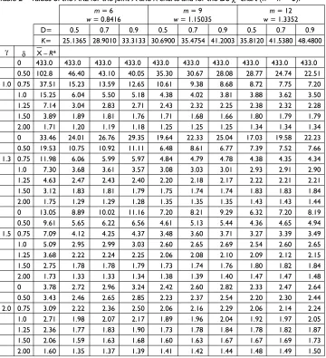
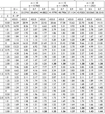
Tables 2 and 3 provide the ARL for the DSχ2 _{chart and for the joint X and R charts. One} can see from these tables that, in most of the cases, the DS χ2 _{chart always detects process} changes faster (lower ARL) than the joint X and R charts. The exceptions occur in some cases when there is a large change in the mean (boldfaced values). For given n, m and d, the ARL for the joint X and R charts and DS χ2 _{chart decreases as} δ _and/or γ _{increases. One} can see from both tables that the ARL value always decreases as n increases.

Table 2 – Values of the ARL for the joint X and R charts and for the DS χ2 _{chart (n = n = 3).}

m = 6 w = 0.8416

m = 9 w = 1.15035

m = 12 w = 1.3352

D= 0.5 0.7 0.9 0.5 0.7 0.9 0.5 0.7 0.9

K= 25.1365 28.9010 33.3133 30.6900 35.4754 41.2003 35.8120 41.5380 48.4800

γ _δ X – R*

0 433.0 433.0 433.0 433.0 433.0 433.0 433.0 433.0 433.0 433.0

0.50 102.8 46.40 43.10 40.05 35.30 30.67 28.08 28.77 24.74 22.51

1.0 0.75 37.51 15.23 13.59 12.65 10.61 9.38 8.68 8.72 7.75 7.20

1.0 15.25 6.04 5.50 5.18 4.38 4.02 3.81 3.88 3.62 3.50

1.25 7.14 3.04 2.83 2.71 2.43 2.32 2.25 2.38 2.32 2.28

1.50 3.89 1.89 1.81 1.76 1.71 1.68 1.66 1.80 1.79 1.79

2.00 1.71 1.20 1.19 1.18 1.25 1.25 1.25 1.34 1.34 1.34

0 33.46 24.01 26.76 29.35 19.64 22.33 25.04 17.03 19.58 22.23

0.50 19.53 10.75 10.92 11.11 6.48 8.61 6.77 7.39 7.52 7.66

1.3 0.75 11.98 6.06 5.99 5.97 4.84 4.79 4.78 4.38 4.35 4.34

1.0 7.30 3.68 3.61 3.57 3.08 3.03 3.01 2.93 2.91 2.90

1.25 4.63 2.47 2.43 2.40 2.20 2.18 2.17 2.22 2.21 2.21

1.50 3.12 1.83 1.81 1.79 1.75 1.74 1.74 1.83 1.83 1.84

2.00 1.75 1.29 1.29 1.28 1.35 1.35 1.35 1.43 1.43 1.44

0 13.05 8.89 10.02 11.16 7.20 8.21 9.29 6.32 7.20 8.19

0.50 9.61 5.65 6.22 6.56 4.61 5.13 5.44 4.36 4.65 4.94

1.5 0.75 7.09 4.12 4.25 4.37 3.48 3.60 3.71 3.27 3.39 3.49

1.0 5.09 2.95 2.99 3.03 2.60 2.65 2.69 2.54 2.60 2.65

1.25 3.68 2.22 2.24 2.25 2.06 2.08 2.10 2.09 2.12 2.15

1.50 2.75 1.78 1.78 1.79 1.73 1.74 1.76 1.80 1.82 1.84

2.00 1.73 1.33 1.33 1.34 1.38 1.39 1.40 1.47 1.47 1.48

0 3.78 2.72 2.96 3.24 2.42 2.60 2.82 2.33 2.47 2.64

0.50 3.43 2.46 2.65 2.85 2.23 2.37 2.54 2.20 2.30 2.44

2.0 0.75 3.09 2.22 2.36 2.50 2.06 2.16 2.29 2.06 2.14 2.24

1.0 2.71 1.98 2.07 2.17 1.89 1.96 2.04 1.92 1.97 2.05

1.25 2.36 1.77 1.83 1.90 1.73 1.78 1.84 1.78 1.82 1.87

1.50 2.06 1.59 1.63 1.68 1.60 1.63 1.67 1.67 1.69 1.73

2.00 1.60 1.35 1.37 1.39 1.41 1.42 1.44 1.48 1.49 1.50

It can be observed from Table 2 that for large disturbances in the mean (δ = 2.0 and in some cases δ = 1.5), the ARL value increases as m increases. The choice of

d affects the speed with which the DS χ2 _{chart signals. In general, larger values of d are} better for detecting shifts in μ with σ = σ0, and worse for detecting increases in σ with μ = μ0. For example, one can see from Table 3, when δ = 0.5, γ = 1.0, as

d increases, the ARL value decreases from 28.94 to 24.74 to 22.42, for m = 10; from 20.66 to 17.38 to 15.62, for m = 15; from 22.70 to 16.82 to 14.15, for m = 20. On the other hand, when δ = 0, γ = 1.5, as d increases, the ARL value increases from 5.85 to 6.77 to 7.77, for m = 10; from 4.77 to 5.50 to 6.36, for m = 15; from 3.85 to 4.28 to 4.88, for m = 20. Table 3 – Values of the ARL for the joint X and R charts and for the DS χ2_{chart (n = n = 5).}

m = 10 w = 0.7665

m = 15 w = 1.0676

m = 20 w = 1.2521

* D = 0.5 0.7 0.9 0.5 0.7 0.9 0.3 0.5 0.7

K = 33.3743 38.6042 44.8822 41.9790 48.7906 57.1134 43.9203 50.0360 58.3310

γ δ X – R*

0 433.0 433.0 433.0 433.0 433.0 433.0 433.0 433.0 433.0 433.0

0.50 56.59 28.94 24.74 22.42 20.66 17.38 15.62 22.70 16.82 14.15

1.0 0.75 16.94 8.26 7.21 6.62 6.02 5.31 4.92 6.38 5.26 4.74

1.0 6.39 3.37 3.07 2.90 2.79 2.62 2.53 3.00 2.78 2.69

1.25 3.07 1.92 1.82 1.77 1.86 1.82 1.80 2.05 2.03 2.02

1.50 1.84 1.41 1.38 1.37 1.51 1.51 1.50 1.67 1.67 1.67

2.00 1.12 1.12 1.12 1.12 1.21 1.21 1.21 1.29 1.29 1.29

0 26.24 16.53 19.09 21.69 13.13 15.42 17.88 9.66 11.25 13.28

0.50 13.23 6.81 6.92 7.05 5.50 5.60 5.70 4.89 4.99 5.11

1.3 0.75 7.33 3.85 3.81 3.79 3.31 3.30 3.29 3.20 3.22 3.24

1.0 4.20 2.46 2.43 2.41 2.31 2.31 2.30 2.37 2.40 2.42

1.25 2.63 1.80 1.79 1.78 1.83 1.84 1.84 1.95 1.97 2.00

1.50 1.84 1.47 1.47 1.47 1.57 1.58 1.59 1.70 1.71 1.72

2.00 1.20 1.20 1.20 1.21 1.30 1.30 1.31 1.38 1.38 1.38

0 9.46 5.85 6.77 7.77 4.77 5.50 6.36 3.85 4.28 4.88

0.50 6.62 3.87 4.16 4.43 3.34 3.59 3.83 3.00 3.19 3.43

1.5 0.75 4.67 2.80 2.92 3.01 2.56 2.68 2.78 2.48 2.58 2.71

1.0 3.25 2.11 2.17 2.21 2.07 2.13 2.18 2.11 2.17 2.25

1.25 2.33 1.70 1.74 1.76 1.76 1.80 1.84 1.86 1.89 1.94

1.50 1.77 1.46 1.49 1.50 1.57 1.59 1.62 1.68 1.69 1.71

2.00 1.24 1.23 1.24 1.25 1.33 1.34 1.35 1.42 1.42 1.42

0 2.64 1.97 2.13 2.33 1.90 2.00 2.14 1.94 1.97 2.03

0.50 2.41 1.83 1.96 2.11 1.81 1.90 2.01 1.87 1.90 1.95

2.0 0.75 2.17 1.70 1.80 1.92 1.73 1.79 1.88 1.81 1.83 1.87

1.0 1.92 1.58 1.65 1.73 1.64 1.69 1.76 1.74 1.75 1.78

1.25 1.69 1.46 1.51 1.58 1.55 1.59 1.64 1.66 1.66 1.68

1.50 1.50 1.37 1.41 1.45 1.48 1.50 1.53 1.58 1.58 1.59

2.00 1.23 1.25 1.26 1.28 1.35 1.36 1.37 1.43 1.43 1.44

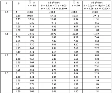
The performance of a control chart can also be measured by the sampling rate. When the joint X and R charts are in use, the sampling rate is given by n (the sample size), and when the DS χ2 _{chart is in use, the sampling rate is given by n (see Equation 2). Like the ARL, the} sampling rate can be used to compare two charts. To keep the comparison meaningful, the two charts should offer the same protection against false alarms by having the same ARL₀. For specifi ed types of process changes, the control chart with the best performance is the one with the lowest sampling rate and best ability of detection. One can see from Table 4 that the DS χ2 _{chart is an interesting alternative to the joint X and R charts, if the aim is} the reduction of the sampling rate. For example, one can see from Table 4, when n = 3.0, δ = 1.0, and γ = 1.3, the DSχ2 _{chart leads to a better trade-off between the time to detect} the process change and the sampling rate required to control the process, that is lower ARL

(5.01 against 7.30), and lower Sampling Rate (1.5 against 3.0).

The Design of the Non-Central Chi-Square Chart with Double Sampling The use of the DS χ2 _{chart requires the specifi cation of d, n}

0, n, and k. According to Equation (2), w is a function of n and n₀. If the practitioners have some idea about the

Table 4 - Values of the ARL for the joint X and R charts and for the DS χ2 _{chart (n} ≠ _n).

γ _δ X – R

n = 3.0

DS χ2 chart n _{= 1.5;} m = 7; d = 0.25 w = 1.7317; k = 21.8140

X – R n = 5.0

DS χ2 chart n _{= 3.0;} m = 11; d = 0.30

w = 1.2816; k = 30.0043

1.0 0 433.0 433.0 433.0 433.0

0.50 102.8 67.58 56.59 39.12

0.75 37.51 22.43 16.94 11.31

1.0 15.25 9.12 6.39 4.56

1.25 7.14 4.62 3.07 2.53

1.50 3.88 2.87 1.84 1.80

1.3 0 33.46 23.90 26.24 15.59

0.50 19.53 12.85 13.23 7.64

0.75 11.98 7.85 7.33 4.60

1.0 7.30 5.01 4.20 3.02

1.25 4.63 3.45 2.63 2.22

1.50 3.12 2.57 1.84 1.80

1.5 0 13.05 9.41 9.46 5.85

0.50 9.61 6.86 6.62 4.23

0.75 7.09 5.15 4.67 3.22

1.0 5.09 3.86 3.25 2.51

1.25 3.68 2.99 2.33 2.05

2.0 0 3.78 3.28 2.64 2.25

0.50 3.43 3.04 2.41 2.12

0.75 3.09 2.79 2.17 1.99

1.0 2.71 2.54 1.92 1.86

1.25 2.36 2.29 1.69 1.69

Table 5 – The ARL and the optimum design parameters for the DS χ2 _charts,

n = n = 3.

δ = 0 δ = 0.5 δ = 1.0

γ γ γ

n0 w d k 1.00 1.25 1.50 1.00 1.25 1.50 1.00 1.25 1.50

15 0 27.580 433 16.8 4.83 66.2 8.99 3.88 6.01 3.47 2.62

15 1 50.649 433 29.6 7.78 18.2 7.91 4.79 3.52 3.07 2.77

15 1.501 0.6 36.628 433 22.8 6.05 22.1 7.83 4.26 3.70 3.09 2.66

15 0.1 27.855 433 17.0 4.87 48.8 8.42 3.84 5.02 3.28 2.56

13 1.423 1 45.936 433 31.1 8.18 19.6 8.25 4.89 3.43 2.99 2.70

10 1.282 1 38.667 433 34.01 9.03 23.2 9.15 5.20 3.47 2.97 2.66

10 0.3 23.424 433 22.2 5.85 39.1 9.28 4.23 4.56 3.19 2.51

Standard X and R charts 433 45.40 13.10 103.00 23.80 9.61 15.30 8.08 5.09

Boldfaced ARL is the minimum one for the specifi ed δ and γ (for which the minimization was per-formed).

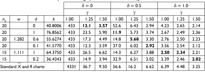
disturbances the process is subject to, then they can use Tables 5 and 6 for selecting the design parameters. These tables provide the values of d, n₀, and k that minimize the average number of samples required to signal δ standard deviation shifts in the process mean accompanied by 100(γ2 _{- 1)% of process variance increase under the constraints that} α≈ 0.0023, n = 3, 3 < n₀≤ 15, and d≤ 1 (Table 5), or n = 5, 5 < n₀≤ 20, and d ≤ 1 (Table 6). For example, Table 6 shows that shifts in the process mean equal to half standard deviation (δ = 0.5), accompanied by 56.25% process variance increase (γ = 1.25) are detected faster when d = 0.6, n₀ = 20, and k = 55.6274.

Comparing Charts

It seems reasonable to compare the DS χ2_{chart and the two-stage sampling (TSS) X and}

R charts in terms of the speed with which they detect process disturbances. When the TSS

X and R charts are in use, samples of size m = n₀ + 1 are taken from the process at regular

Table 6 – The ARL and the optimum design parameters for the DS χ2 _{charts, n = n = 5.}

δ = 0 δ = 0.5 δ = 1.0

γ γ γ

n₀ w d k 1.00 1.25 1.50 1.00 1.25 1.50 1.00 1.25 1.50

20 0 40.8006 433 12.1 3.57 52.6 6.43 2.94 4.23 2.65 2.14

20 1 76.8562 433 23.5 5.90 11.9 5.73 3.74 2.67 2.49 2.36

20 1.282 0.6 55.6274 433 17.3 4.49 14.8 5.68 3.30 2.76 2.50 2.23

20 0.1 41.5770 433 12.3 3.59 37.0 6.02 2.92 3.56 2.54 2.12

15 1.111 1 64.3750 433 26.5 6.62 14.3 6.27 3.88 2.50 2.34 2.21

15 0.2 36.4343 433 14.9 3.94 32.9 6.51 3.02 3.39 2.46 2.02

Standard X and R charts 433† 36.7 9.50 56.6 16.2 6.62 6.39 4.48 3.25

time intervals. The sampling is performed in two stages. During the fi rst stage, the fi rst item of the sample is inspected. If its X value is close to the target value (|X – μ0|< wσ0, w > 0), then the sampling is interrupted. Otherwise, the sampling goes on to the second stage, where the remaining n₀ items are inspected and the X and R values are computed. The signal is given by an X value beyond the control limits (n0!kXv0/ n0) and/or by an

R value above the upper control limit, k_R(n₀)σ0. The sample values can be computed taking into account all m values (DS procedure), or only the remaining n₀values (TSS procedure). The DS charts are more effective in detecting process disturbances. This result is intuitive, once the DS scheme makes better use of the sample information. Table 7 provides the

ARL for the DS χ2 _{chart and for the TSS X and R charts. One can see from this table that}

the chi-square chart competes with the joint charts. Thus, a single chart can be used for

monitoring both the process mean and variance.

Very recently, Reynolds and Stoumbos (2004) investigated the use of two EWMA

charts or two CUSUM charts for monitoring the mean and the variance. In their study, the

EWMA_X chart for detecting changes in μ is based on the control statistic

EX

k = (1 – λ)E X

k-1 + λXk , k = 1, 2,..., (4)

where: λ is a tuning parameter satisfying 0 < λ≤ 1 and the starting value is usually taken to be EX

0 = μ0. A signal is given at sample k if E X

k falls outside the control limits

/( ( ))

hEX n 2

0! 0

n m -m v (5)

where: m/( (n 2-m v)) 0 is the asymptotic in-control standard deviation of E

X k. The

EWMA_X2 chart for detecting changes in σ is based on the control statistic

( )max , , , ,...,

Ek 1 E X _n k 1 2

X k X ki i n 1 0 2 0 2 1 2 2

m v m n

= - - + - =

=

_ i

$ .

_!

where: EX2 0 = σ

2

0 . A signal is given at sample k if E X2 0

falls above the control limit

/( ( ))

hEX 2 n 2

0 2

0 2

2

v + m -m v (7)

Table 7 – Values of theARL for the TSS X and R Charts and for the DS χ2_{chart (n= n = 5;n} 0 = 14;

w = 1.068).

TSS X and R charts* kX = 2.873; kR(n0) = 5.725

DS χ2_chart k = 42.6115; d = 0.7

δ δ

γ 0.00 0.50 0.75 1.00 1.25 1.50 γ 0.00 0.50 0.75 1.00 1.25 1.50

1.0 433.0 18.01 5.13 2.51 1.78 1.49 1.0 433.0 17.38 5.17 2.62 1.82 1.51

1.3 19.29 7.50 3.88 2.42 1.82 1.55 1.3 15.42 5.60 3.30 2.31 1.84 1.58

1.5 6.57 4.33 3.02 2.22 1.79 1.56 1.5 5.50 3.59 2.68 2.13 1.80 1.59

2.0 2.13 1.99 1.85 1.71 1.59 1.49 2.0 2.00 1.90 1.79 1.69 1.59 1.50

The CUSUM_X chart for detecting changes in μ is based on two separate one-side CUSUM statistics. The upper CUSUM statistic for detecting increases in μ is

, / , , ,...,

max

Ck 0 C X 2 k 1 2

X

k X

k

1 n0 g v0

= + - - n =

+

-+ _ i

# - (8)

and the lower CUSUM statistic for detecting decreases in μ is:

, / , , ,...,

min

Ck 0 C X 2 k 1 2

X

k X

k

1 n0 g v0

= + - + n =

-- _ i

# - (9)

The initial values for the statistics are CX+ 0 = C

X-0

= 0. The chart parameter ζμ is defi ned as

ζμ = |μ1 – μ2|/σ, where μ1 is an out-of-control value of μ that should be detected quickly.

The chart signals if:

> /

Ck h n

X

CXv0

+ _or

< /

Ck h n

X

CXv0

-- ₍₁₀₎

The CUSUM_X2 chart for detecting changes in σ is based on the control statistic:

, , , ,...,

max

C 0 C X _n n k

1 21 1 2 k X k X ki 1 0 2 2 0 2

2 2 n

g g

v

= + -

-- v =

v

-

-_

f i p

$ .

_!

where CX2

0 = 0 and the upper control limit is

h_CX2 σ2

0/n (12)

The chart parameter ζ_σ is defi ned as ζ_σ = σ1/σ0, where σ1 (σ1 > σ0) is a value of σ that should be detected quickly.

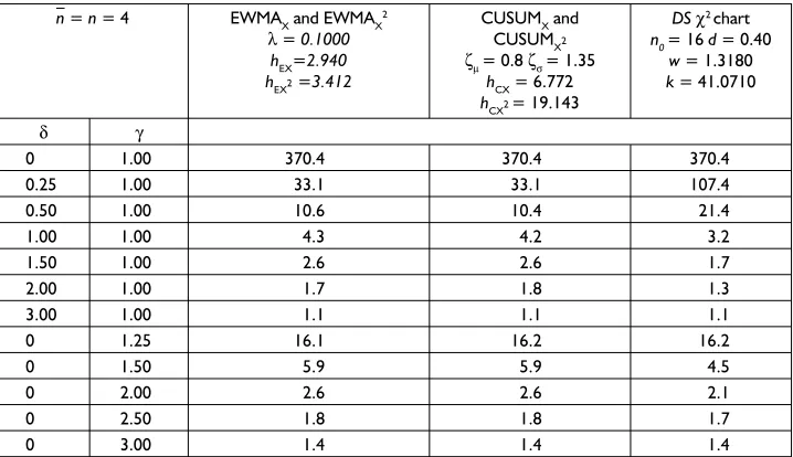
Comparing the EWMA and the CUSUM chart combinations with the corresponding

DS Chi-square chart in Table 8 shows that the EWMA and the CUSUM chart combinations are

better for small shifts in μ, but the DS χ2 _{chart is equivalent or slightly better for changes} in σ ranging from γ = 1.25 to γ = 3.00.

Illustrative Example

The joint X and R charts have been used to monitor the diameter of shafts. As the specifi cations of the diameters (0.7500 ± 0.0030 inches) are very tight, a minor shift in the process mean accompanied by increases in the variance leads to the manufacturing of a large number of shafts with diameters beyond the specifi cations. Past data show that the standard deviation (σ) of the diameters, originally stable at σ0 = 0.0012 inches, increases when the process mean goes off-target. The parameters of the joint charts are n = 3,

k_X = 3.250 and k_R(n) = 5.009. The Double Sampling Non-Central Chi-Square Chart was designed to replace the joint charts. At the fi rst stage, one item of the sample is inspected. If its X value belongs to the interval μ0 ± wσ0 (w = 1.3352), then the sampling is interrupted. Otherwise, at the second stage, the remaining sample items are inspected,

T Xj 0 0

2

n pv

From Table 2, one can see that the DS χ2 _{chart detects process disturbances faster than} the joint X and R charts. For instance, to detect mean shifts of half standard deviation (δ = 0.5) accompanied by 69% of process variance increase (γ = 1.3), the DS χ2 _{chart, with}

n₀ = 11 and d = 0.7, requires, on average, 7.52 samples (ARL = 7.52), against 19.53 samples (the ARL value for the joint X and R charts with n = 3, k_X = 3.250 and k_R(n) = 5.009).

During the in-control period, approximately 82% of the two stage procedure does

not go to the second stage (that is, Pr[|Z|< w = 1.335|Z≈N(0,1)] ≈ 0.82); consequently, most of the time the user will not have to measure the diameter of any shaft. As the process is very stable (remains in control most of the time) the occurrence of X or R

values outside the control limits is rare. The activity of measuring three shafts at each hour plus computation of X and R values may be considered tedious. The DS procedure provides some relief once the average length of the interval between no-interrupted

samplings (when measurements are effectively required) is longer than 5 hours and half (1/0.18 sampling intervals of one hour). Hence, most of the time, measurements will be performed once or twice per day (considering 8 hours of labor). One can raise the

question that it is more monotonous to deal with the non-central chi-square statistic than with X and R statistics, however, with a programmable calculator, the required number of keystrokes to obtain the T values or the X values is just the same. In summary,

the DS χ2 _{chart is not only more sensitive than the joint X and R charts, but operationally} simpler as well.

Table 8 – ARL for the EWMA and CUSUM chart combinations and for the DS χ2 _chart.

n = n = 4 EWMAX and EWMAX 2 λ = 0.1000

hEX=2.940 hEX2 =3.412

CUSUMX and CUSUM_X2 ζμ = 0.8 ζσ = 1.35

hCX = 6.772 h_CX2= 19.143

DS χ2 _chart n₀ = 16 d = 0.40

w = 1.3180 k _{= 41.0710}

δ γ

0 1.00 370.4 370.4 370.4

0.25 1.00 33.1 33.1 107.4

0.50 1.00 10.6 10.4 21.4

1.00 1.00 4.3 4.2 3.2

1.50 1.00 2.6 2.6 1.7

2.00 1.00 1.7 1.8 1.3

3.00 1.00 1.1 1.1 1.1

0 1.25 16.1 16.2 16.2

0 1.50 5.9 5.9 4.5

0 2.00 2.6 2.6 2.1

0 2.50 1.8 1.8 1.7

Conclusions

In this paper we have shown that it is possible to design one chart, which can monitor both the process mean and variance. The DS χ2 _{control chart is of particular interest when} the quality characteristic can be evaluated either by attribute or variable. As it is much easier to deal with attributes than with variables the proposed chart is a valuable tool. A classical example consists in monitoring the diameter of shafts. During the fi rst stage of the sampling, a gauge is used to decide if the whole sample must be inspected by variable (for instance, using a micrometer) or if the sampling must be interrupted. This two-stage procedure has two advantages. The fi rst advantage is the reduced number of times the user will need to perform measurements, and the second is the gain in speed with which process disturbances will be detected. The DS χ2 _{chart was conceived to be a practical tool} for surveillance of processes subject to small to moderate disturbances. Moreover, when the process is stable, and the joint X and R charts are in use, the monitoring becomes monotonous because an X or a R values rarely falls outside the control limits. The natural consequence is that the user pays less and less attention to the steps required to obtain the X and R value. But in some cases, this lack of attention can result in serious mistakes. When the DS χ2 _{chart is in use, most of the samplings are interrupted, consequently,} most of the time the user will be working with attributes. Our experience shows that the inspection of one item by attribute is much less monotonous than measuring three, four or fi ve items at each sampling.

Acknowledgment

The fi nancial support of this joint work was provided in part by CNPq (the Brazilian Council for Scientifi c and Technologic Development). Its assistance is gratefully acknowledged.

References

Albin, S. L., Kang, L. and Sheha, G. (1997). An X and EWMA Chart for Individual Observations. Journal of Quality Technology, v. 29, p. 41-48.

Amin, R. W. and Miller, R. W.(1993). A Robustness Study of X Charts with Variable Sampling Intervals. Journal of Quality Technology, v. 25, p. 36-44.

Chen, G., Cheng, S. W. and Xie, H. (2001). Monitoring Process Mean and Variability with One EWMA Chart. Journal of Quality Technology, v.33, p. 223-233.

Chen, G., Cheng, S. W. and Xie, H. (2004). A New EWMA Control Chart for Monitoring Both Location and Dispersion. Quality Technology & Quantitative Management, v. 1, n. 2, p. 217-231.

Costa, A. F. B. (1997). X Charts with Variable Sample Size and Sampling Intervals. Journal of Quality Technology, v. 29, p.197-204.

Costa, A. F. B. (1998a). VSSI X Charts with Sampling at Fixed Times. Communications in Statistics – Theory and Methods, v. 27, n. 11, p. 2853-2869.

Costa, A. F. B. (1998b). Joint X and R charts with Variable Parameters. IIE-Transactions, v. 30, n. 11, p.505-514.

Costa, A. F. B. (1999a). X Charts with Variable Parameters. Journal of Quality Technology, v. 31, n. 4, p. 408-416.

Costa, A. F. B. (1999b). Joint X and R charts with Variable Sample Sizes and Sampling Intervals. Journal of Quality Technology, v. 31, n. 4, p. 387-397.

Costa, A. F. B. (1999b). X Charts with Supplementary Samples to Control the Mean and Variance. International Journal of Production Research, v. 38, n. 16, p. 3801-3809. Costa, A. F. B. and Rahim, M. A.(1999b). Economic Design of X and R Charts Under Weibull

Shock Models. Quality and Reliability Engineering International, v. 16, p.143-156, X. Costa, A. F. B., Rahim, M. A. (2004). Joint X and R Charts with Two Stage Samplings. Quality

andReliability Engineering-International, v. 20, n. 7, p. 699-708.

Croasdale, R. (1974). Control Charts for a Double-Sampling Scheme Based on Average Production Run Length. International Journal of Production Research, v.12, p.585-592.

Das, T. K., Jain, V. and Gosavi, A. (1997). Economic Design of Dual-Sampling Interval Policies for X Charts With and Without Run Rules, v. 29, p. 497-506.

Daudin, J. J. (1992). Double Sampling X Charts. Journal of Quality Technology, v. 24, p. 78-87.

De Magalhães, M. S., Epprecht, E. K. and Costa, A. F. B. (2001). Economic Design of a Vp X Chart. International Journal of Production Economics, v. 74, p.191-200.

De Magalhães, M. S., Costa, A. F. B. and Epprecht, E. K. (2002). Constrained Optimization Model for the Design of an Adaptive X Chart. International Journal of Production Research, v.40, p. 3199-3218.

De Magalhães, M. S. and Moura Neto, F. D. (2005). Joint Economic Model for Totally Adaptive X and R Charts. European Journal of Operation Research, v. 161, p.148-161, . Domangue, R. and Patch, S. C. (1991). Some Omnibus Exponentially Weighted Moving

Average Statistical Process Monitoring Schemes. Technometrics, v. 33, n. 3, p. 299-313.

Epprecht, E. K. and Costa, A. F. B. (2001). Adaptive Sample Size Control Charts for Attributes. Quality Engineering, v. 13, n. 3, p. 465-473.

Epprecht, E. K., Costa, A. F. B. and Mendes F. C. T. (2003). Adaptive Control Charts for Attributes. IIE Transactions, v. 35, n. 6, p. 567-582.

Lin, Y. C. and Chou, C. Y. (2005). Adaptive X Control Charts with Sampling at Fixed Times. Quality and Reliability Engineering International(in press).

Park, C. and Reynolds, M. R., Jr. (1994). Economic Design of a Variable Sample Size X-Chart. Communications in Statistics-Simulation and Computation, v. 23, p.467-483. Park, C. and Reynolds, M. R., Jr. (1999). Economic Design of a Variable Sampling Rate

X-Chart. Journal of Qual+ity Technology, v.31, p.427-443.

Prabhu, S. S., Montgomery, D. C. and Runger, G. C. (1994). A Combined Adaptive Sample Size and Sampling Interval X Control Scheme. Journal of Quality Technology, v.26, p.164-176.

Prabhu, S. S., Montgomery, D. C. and Runger, G. C. (1997). Economic-Statistical Design of an Adaptive X Chart. International Journal of Production Economics, v. 49, p.1-15.

Prabhu, S. S., Runger, G. C. and Keats, J. B. (1993). An Adaptive Sample Size X Chart. International Journal of Production Research, v. 31, p. 2895-2909.

Rahim, M. A., Costa, A. F. B. (2000). Joint Economic Design of X and R Charts Under Weibull Shock Models. International Journal of Production Research, v. 28, p. 2871-2889. Reynolds, M. R. (1996a). Variable-Sample-Interval Control Charts with Sampling at Fixed

Times. IIE Transactions, v. 28, p. 497-510.

Reynolds, M. R., Jr. (1996b). Shewhart and Ewma Variable Sampling Interval Control Charts with Sampling at Fixed Times. Journal of Quality Technology, v. 28, p.199-212.

Reynolds, M. R., Jr., Amin, R. W. and Arnold, J. C. (1990). Cusum Charts with Variable Sampling Intervals. Technometrics, v. 32, p.371-384.

Reynolds, M. R, Jr., Amin, R. W., Arnold, J. C. and Nachlas, J. A. (1988). X Charts with Variable Sampling Intervals. Technometrics, v. 30, p.181-192.

Reynolds, M. R., Jr. and Stoumbos, Z. G. (2001). Monitoring the Process Mean and Variance Using Individual Observations and Variable Sampling Intervals. Journal of Quality Technology, v. 33, p.181-205.

Reynolds, M. R., Jr. and Stoumbos, Z. G. (2004). Control Charts and the Effi cient Allocation of Sampling Resources. Technometrics, v. 46, n. 2, p.200-214.

Runger, G. C. and Montgomery, D. C.(1993). Adaptive Sampling Enhancements for Shewhart Control Charts. IIE Transactions, v. 25, p.41-51.

Runger, G. C. and Pignatiello, J. J, Jr. (1991). Adaptive Sampling for Process Control. Journal of Quality Technology, v. 23, p.135-155.

Saccucci, M. S., Amin, R. W. and Lucas, J. M. (1992). Exponentially Weighted Moving Average Control schemes with variable sampling intervals. Communication in Statistics – Simulation and Computation,v.21, p. 627-657.

Biography

Antonio F. B. Costa is a Professor in the Department of Production at UNESP- São Paulo State University, Brazil. He was a postdoctoral fellow in the Center for Quality and Productivity Improvement at University of Wisconsin, Madison, USA. His current interest is in statistical quality control. He has published papers in the Brazilian Journal of Operations & Production Management, Journal of Quality Technology, Communications in Statistics, IIE Transactions, International Journal of Production Research, International Journal of Production Economics, Quality and Reliability Engineering International, Quality Technology and Quantitative Management, Journal of Applied Statistics, European Journal of Operation Research, Quality Engineering, Journal of Quality in Maintenance Engineering and (in Portuguese) in Gestão & Produção

and Pesquisa Operacional. He received a Best Paper Award from IIE Transactions. He is

a Certifi ed Quality Engineer by the American Society for Quality. He is a member of the

Associação Brasileira de Engenharia de Produção (ABEPRO) and of the Sociedade Brasileira

de Pesquisa Operacional (SBPO).

Maysa S. De Magalhães is an Associate Professor in the Escola Nacional de Ciências Estatísticas at Instituto Brasileiro de Geografi a e Estatística, Rio de Janeiro, Brazil. She received a PhD degree from Pontifícia Universidade Católica do Rio de Janeiro. Her current interests are in statistical quality control and times series. She has published papers in the Brazilian Journal of Operations & Production Management, International Journal of Production Economics, European Journal of Operational Research, International Journal of Production Research, Quality and Reliability Engineering International, and (in Portuguese) in Gestão & Produção. She is a member of the Sociedade Brasileira de Pesquisa

Operacional (SBPO).

Eugenio Kahn Epprecht is an Associate Professor in the Department of Industrial Engineering at the Pontifícia Universidade Católica (PUC), Rio de Janeiro, Brazil. He received his Engineering and MSc degrees from PUC, Rio de Janeiro, and his Ph.D. from

the Facultés Universitaires Notre-Dame de la Paix, Belgium. His chief research interests are

statistical quality control and industrial applications of statistics and operations research. He has published papers in the Brazilian Journal of Operations & Production Management, IIE Transactions, International Journal of Production Research, International Journal of Production Economics, Quality Engineering, and (in Portuguese) in Gestão & Produção,

Pesquisa Operacional and Pesquisa Naval. He is a member of the American Society for

Quality (ASQ), of the Associação Brasileira de Engenharia de Produção (ABEPRO) and of the

Appendix: Computation of the Risk α and the Power of the Control Chart 1-β. The statistic T is given by:

, ,...

T Xj i 1 2

j m 0 0 2 1 n pv = - + = = _ i

!

Xj X

j m

0 0 2

1 0 0 2 2

n pv n pv

= - + + - +

=

_ i _ i

!

Xj X n X X

j m

2

0 0 2

1 0 0 2 2

n pv n pv

= - + - + + - +

=

_ i _ i _ i

!

Xj X n X X

j m

2

0 0 0 0 0 2

1 0 0 0 0 2 2

n dv dv pv n dv dv pv

= - + - - + + + - - + +

=

_ i _ i _ i

!

where: X Xj j

m

2

=

=

!

/

T Xj X Z n Z

j m 1 2 1 2 2 0 2 1 2

v = _v- + + d_c+p + + d_c+p

=

e o e o e o

!

where: Z n0 X 0 0 0

cv

n dv

= - - ~N (0,1) and Z1 X

0 1 0 0

cv

n dv

= - - ~N (0,1). Therefore,

during the out-of-control period, the fi rst term on the right side of Equation (A₁) follows a chi-square distribution with m-2 degrees of freedom; the second term follows a non-central chi-square distribution with 1 degree of freedom and non-non-centrality parameter λ = n₀[(δ + ξ)/γ]2_{. Consequently, the sum of these fi rst and second terms follows a} chi-square distribution with n₀ degrees of freedom and non-centrality parameter λ = n₀[(δ + ξ)/γ]2_{. To obtain} α _{and 1-}β_{, we consider the Equation (3)}

[( > ) ( > )] ( > ) ( > )

Pr Pr

Q X1 0 w 0 T k 0 Z w T k

2

1

1 2 2

+ +

n v v _cd _c

v c

= - = = + G

> > [| |> ]

Pr T k Z w Pr Z w

1

2 2 1 1

v c c

d

c cd c

= = + G + =

Then, using Equation A₁, we have:

{ >[ ( ) ]}

Pr

Q k z d e dz

2

, [( )/ ]

( )/ .

n n d

w z

2

2

2 0 5

0 0 2

2 | c c d r = - + - +

3 d c

d c

-- -

-#

{ >[ ( ) ]}

Pr k z d e dz

2

, [( )/ ] ( )/

.

n n d w

z

2

2

2 0 5

0 0 2

2 | c c d r - + + 3 d c

d c +

-#