Optimal Hitting Sets for Combinatorial Shapes

www.theoryofcomputing.org

SPECIAL ISSUE: APPROX-RANDOM 2012

Optimal Hitting Sets for

Combinatorial Shapes

∗

Aditya Bhaskara

Devendra Desai

Srikanth Srinivasan

Received November 5, 2012; Revised April 16, 2013; Published May 25, 2013

Abstract: We consider the problem of constructing explicit Hitting Sets forcombinatorial shapes, a class of statistical tests first studied by Gopalan, Meka, Reingold, and Zuckerman (STOC 2011). These generalize many well-studied classes of tests, including symmetric functions and combinatorial rectangles. Generalizing results of Linial, Luby, Saks, and Zuck-erman (Combinatorica 1997) and Rabani and Shpilka (SICOMP 2010), we construct explicit hitting sets for combinatorial shapes of size polynomial in the alphabet size, dimension, and the inverse of the error parameter. This is optimal up to polynomial factors. The best previous hitting sets came from the pseudorandom generator construction of Gopalan et al., and in particular had size that was quasipolynomial in the inverse of the error parameter.

Our construction builds on natural variants of the constructions of Linial et al. and Rabani and Shpilka. In the process, we construct fractional perfect hash families and hitting sets for combinatorial rectangles with stronger guarantees. These might be of independent interest.

ACM Classification:F.1.2, F.1.3

AMS Classification:68Q10, 68Q15, 68R10, 68W20

Key words and phrases:derandomization, expanders, explicit construction, hitting sets, perfect hashing

∗_{An earlier version of this paper appeared in theProceedings of the 16th International Workshop on Randomization and}

1

Introduction

Randomness is a tool of great importance in computer science and combinatorics. The probabilistic method is highly effective both in the design of simple and efficient algorithms and in demonstrating the existence of combinatorial objects with interesting properties. But the use of randomness also comes with some disadvantages. In the setting of algorithms, introducing randomness adds to the resource requirements of the algorithm, since truly random bits are hard to come by. For combinatorial constructions, explicitversions of these objects often turn out to have more structure, which yields advantages beyond the mere fact of their existence (e. g., we know of explicit error-correcting codes that can be efficiently encoded and decoded, but we do not know of an analogue for random linear codes [7]). Thus, it makes sense to ask exactly how powerful probabilistic algorithms and arguments are. Can they be “derandomized,” i. e., replaced by deterministic algorithms/arguments of comparable efficiency?1 There is

a long line of research that has addressed this question in various forms [22,13,21,26,19].

An important line of research in this area is the question of derandomizing randomized space-bounded algorithms. In 1979, Aleliunas et al. [1] demonstrated the power of these algorithms by showing that undirected s-t connectivity can be solved by randomized algorithms in justO(logn) space. In order to show that any randomizedLOGSPACEcomputation could be derandomized within the same space requirements, researchers considered the problem of constructing an efficientε-pseudorandom

generator(ε-PRG) that would stretch a short random seed to a long pseudorandom string which would

be indistinguishable (up to errorε) from strings chosen from the uniform distribution to anyLOGSPACE

algorithm.2 In particular, anε-PRG (for small constantε>0) with seed lengthO(logn)would allow

efficient deterministic simulations ofLOGSPACErandomized algorithms since a deterministic algorithm could run over all possible random seeds.

A breakthrough work of Nisan [21] took a massive step towards this goal by giving an explicit

ε-PRG forε=1/poly(n)that stretchesO(log2n)truly random bits to ann-bit pseudorandom string for

LOGSPACEcomputations. In the two decades since, however, Nisan’s result has not been improved upon at this level of generality. However, many interesting sub-cases of this class of functions have been considered as avenues for progress [23,15,17,16,14].

In this work, we consider a very natural class of functions known ascombinatorial shapes. A Boolean function f is an(m,n)-combinatorial shape if it takesninputsx1, . . . ,xn∈[m]and computes a symmetric

function of Boolean bitsyi that depend on the membership of the inputs xi in setsAi ⊆[m], called accepting sets, associated with f. (A function of Boolean bitsy1, . . . ,ynis symmetric if and only if the

output depends only on the sum of the input bits.) In particular, ANDs, ORs, modular sums and majorities of subsets of the input alphabet all belong to this class. Until recently, Nisan’s result gave the best known seed length for any explicitε-PRG for this class, even whenε was a constant. In 2011, however, Gopalan

et al. [11] gave an explicitε-PRG for this class with seed lengthO(log(mn) +log2(1/ε)). This seed

length is optimal as a function ofmandnbut suboptimal as a function ofε, and for the very interesting

case ofε =1/nO(1), this result does not improve upon Nisan’s work.

Is the setting of small error important? We think the answer is yes, for many reasons. The first deals

1_{A “deterministic argument” for the existence of a combinatorial object is one that yields an efficient deterministic algorithm}

for its construction.

with the class of combinatorial shapes: many tests from this class accept a random input only with inverse polynomial probability (e. g., the alphabet is{0,1}and the test accepts iff the Hamming weight of itsn

input bits isn/2); for such tests, the guarantee that a 1/no(1)-PRG gives us is unsatisfactory. Secondly, while designing PRGs for some class of statistical tests with (say) constant error, it often is the case that one needs PRGs with much smaller error—e. g., one natural way of constructing almost-lognwise independent spaces uses PRGs that fool parity tests [20] to within inverse polynomial error. Thirdly, the reason to improve the dependence on the error is simply because we know that such PRGs exist. Indeed, a randomly chosen function that expandsO(logn)bits to ann-bit string is, w.h.p., anε-PRG

forε=1/poly(n). Derandomizing this existence proof is a basic challenge in understanding how to eliminate randomness from existence proofs. The tools we gain in solving this problem might help us in solving others of a similar flavor.

Our result Constructing optimal PRGs is usually a hard problem, but there is a well-studied weakening that we consider in this paper: constructing smallε-hitting sets(ε-HS). Anε-HS for a class of functions

has the property that any function from that class that accepts at least anεfraction of uniformly random strings accepts at least one of the strings in the hitting set. This is clearly a weaker guarantee than what an

ε-PRG gives us. Nevertheless, in many cases, this problem turns out to be very interesting and non-trivial.

In particular, a polynomial sized andLOGSPACE computableε-HS for the class of space-bounded

computations would solve the long-standing open question of whetherRL=L.

Our main result is an explicitε-HS of size poly(mn/ε)for the class of combinatorial shapes, which

isoptimal, to within polynomial factors, for all errors. Here,explicitmeans that it can be constructed by a deterministic algorithm in time poly(mn/ε)and spaceO(logm+logn+log(1/ε)).

Theorem 1.1(Main Result (informal)). For any m,n∈_N,ε>0, there is an explicitε-HS for the class of

combinatorial shapes of sizepoly(mn/ε).

Related work As far as we know, ours is the first work to specifically study the problem of constructing hitting sets for combinatorial shapes. However, there has been a substantial amount of research into both PRGs and hitting sets for many interesting subclasses of combinatorial shapes, and also some generalizations.

Naor and Naor [20] constructedε-PRGs for parity tests of bits (alphabet size 2) with a seed length

ofO(logn+log(1/ε))that is optimal up to a constant factor [4]; these results were extended by Lovett,

Reingold, Trevisan, and Vadhan [16] and Meka and Zuckerman [18] to modular sums (with coefficients) and separately by Watson [27] to parity sets over a larger alphabet, though with suboptimal seed length. Combinatorial rectangles, another subclass of combinatorial shapes, have also been the subject of much attention. A series of works [8,6, 17] have constructedε-PRGs for this class of functions:

the best such PRG, due to Lu [17], has seed lengthO(logn+log3/2(1/ε)). Linial, Luby, Saks, and

Zuckerman [15] constructed optimal hitting sets for this class of tests. We build on many ideas from this work.

We also mention two more recent results that are very pertinent to our work. The first has to do with

use a bucketing and expander walk construction to build their hitting set. Our construction uses similar ideas.

The final result that we use is the PRG for combinatorial shapes by Gopalan et al. [11] that was mentioned in the introduction. This work directly motivates our results and moreover, we use their PRG as a black-box within our construction.

2

Preliminaries

Definition 2.1(Combinatorial shapes, rectangles, and thresholds). A function f :[m]n_{→ {0,1}is an}

(m,n)-combinatorial shapeif there exist setsA1, . . . ,An⊆[m]and a symmetric functionh:{0,1}n→ {0,1}such that f(x1, . . . ,xn) =h(1A1(x1), . . . ,1An(xn)).

3 _{Ifhis the AND function, we call f an(m,n)}

-combinatorial rectangle. Ifh is an unweighted threshold function, i. e., h accepts iff∑i1Ai(xi)≥θ

for someθ∈N, then f is said to be an(m,n)-combinatorial threshold. We denote byCShape(m,n),

CRect(m,n), andCThr(m,n)the class of(m,n)-combinatorial shapes, rectangles, and thresholds respec-tively.

Notation In many arguments, we will work with a fixed collection of accepting setsA₁, . . . ,An⊆[m]

that will be clear from the context. In such a scenario, fori∈[n], we letXi=1Ai(xi)and denote byX

the corresponding membership vector, i. e., the bits(X1, . . . ,Xn). Fori∈[n], letpi=|Ai|/m,qi=1−pi

andwi=piqi. Define theweightof a shape f asw(f) =∑iwi. Also letµ(f):=∑ipi. Forθ∈N, let

Tθ :{0,1}n→ {0,1}be the symmetric function that accepts iff the sum of its inputs is at leastθ.

Definition 2.2(Pseudorandom generators and hitting sets). LetF⊆ {0,1}D_{denote a Boolean function}

family for some input domainD. A functionG:{0,1}s_{→Dis an}

ε-pseudorandom generator (ε-PRG)

with seed lengthsfor a class of functionsFif for all f ∈F,

Pr

x∈u{0,1}s

[f(G(x)) =1]− Pr

y∈uD

[f(y) =1]

≤ε.

Anε-hitting set (ε-HS) forFis a multi-setH containing only elements fromDs.t. for any f ∈F, if

Prx∈uD[f(x) =1]≥ε, then∃x∈Hsuch that f(x) =1.

Remark 2.3. Whenever we say that there existexplicitfamilies of combinatorial objects of some kind, we mean that the object can be constructed by a deterministic algorithm in time polynomial and space logarithmic in the description of the object. It will be clear from the formal descriptions of the hitting sets that they can be constructed this efficiently.

We will use the following known results in our constructions.

Theorem 2.4(ε-PRGs forCShape(m,n)[11]). For everyε>0, there exists an explicitε-PRGGm_GMRZ,n,ε :

{0,1}s_→[m]n_{forCShape(m,n)with seed length s=O(log(mn) +log}2_(1/

ε)).

Theorem 2.5(ε-HSforCRect(m,n)[15]). For everyε>0, there exists an explicitε-hitting setSm_LLSZ,n,ε

forCRect(m,n)of sizepoly(m(logn)/ε).

3₁

We will also need a stronger version ofTheorem 2.5for special cases of combinatorial rectangles. Informally, the strengthening says that if the acceptance probability of a “nice” rectangle is>pfor some

reasonably large p, then a close topfraction of the strings in the hitting set are accepting. Formally, the following is proved later in the paper.

Theorem 2.6(StrongerHSforCRect(m,n)). For all constants c≥1, m=nc, andρ≤clogn, there is an explicit setSn_rect,c,ρof size nOc(1)_{such that for any}R_{∈CRect(m,n)which satisfies the properties:}

1. Ris defined by Ai, and the rejecting probabilities qi:= (1− |Ai|/m)which satisfy∑iqi≤ρ,

2. Prx∼[m]n[R(x) =1]≥p (≥1/nc)

we have

Pr

x∼_Sn_rect,c,ρ

[R(x) =1]≥ p

2Oc(ρ).

Recall that a distributionµover[m]nisk-wise independent fork∈Nif for anyS⊆[n]such that|S| ≤k, the marginalµ|Sis uniform over[m]|S|. Also,G:{0,1}s→[m]nis ak-wise independent probability space over[m]n_{if for uniformly randomly chosenz∈ {0,1}}s_{, the distribution ofG(z)isk-wise independent.}

Fact 2.7 (Explicit k-wise independent spaces, [2]). For any k,m,n∈_N, there is an explicit k-wise independent probability spaceGm_k-wise,n :{0,1}s_→[m]n_{with s=O(klog(mn)).}

We will also use the following result of Even et al. [8].

Theorem 2.8. Fix any m,n,k∈_N. Then, if f ∈CRect(m,n)andµis any k-wise independent distribution over[m]n, then we have

Pr

x∈[m]n[f(x) =1]−x∼µPr[f(x) =1]

≤ 1

2Ω(k).

Expanders Recall that a degree-DmultigraphG= (V,E)onNvertices is an(N,D,λ)-expander if the

second largest (in absolute value) eigenvalue of its normalized adjacency matrix is at mostλ. We need

the expander graph to be regular in theweightedsense, i. e., the uniform distribution should be the graph’s stationary distribution. We will use explicit expanders as a basic building block. We refer the reader to the excellent survey of Hoory, Linial, and Wigderson [12] for various related results.

Fact 2.9(Explicit expanders [12]). Given anyλ>0and N∈N, there is an explicit(N,D,λ)-expander

where D= (1/λ)O(1).

Expanders have found numerous applications in derandomization. A central theme in these appli-cations is to analyze random walks on a sequence of expander graphs. LetG₁, . . . ,G<sub>`</sub>be a sequence of (possibly different) graphs on thesamevertex setV. AssumeGi(i∈[`]) is an(N,Di,λi)-expander. Fix

anyu∈V andy1, . . . ,y`∈Nsuch thatyi∈[Di]for eachi∈[`]. Note that(u,y1, . . . ,y`)naturally defines

a “walk”(v₁, . . . ,v<sub>`</sub>)∈V`as follows:v₁is they₁th neighbor ofuinG₁and for eachi>1,viis theyith

neighbor ofvi−1inGi. We denote byW(G1, . . . ,G`)the set of all tuples(u,y1, . . . ,y`)as defined above.

Moreover, givenw= (u,y1, . . . ,y`)∈W(G1, . . . ,G`), we definevi(w)to be the vertexvidefined above

We need a variant of a result due to Alon, Feige, Wigderson, and Zuckerman [3]. The lemma as it is stated below is slightly more general than the one given in [3] but it can be obtained by using essentially the same proof and setting the parameters appropriately.

Lemma 2.10. Let G₁, . . . ,G<sub>`</sub>be a sequence of graphs defined on the same vertex set V of size N. Assume that Giis an(N,Di,λi)-expander. Let V1, . . . ,V`⊆V such that|Vi| ≥piN>0for each i∈[`]. Let p0=1.

Then, as long as for each i∈[`],λi≤(pipi−1)/8,

Pr

w∈_W(G1,...,G`)

[∀i∈[`],vi(w)∈Vi]≥(0.75)`

_∏

i∈[`]

pi. (2.1)

Actually, the way we have defined our walk, we do not need the graphG1. It is there in the statement

just to make the notation simpler. In our applications, it is convenient to use the following corollary.

Corollary 2.11. Let V be a set of N elements, and let0<pi<1for1≤i≤`be given. There exists an explicit set of walksW, each of length`, such that for any subsets V1,V2, . . . ,V`of V , with|Vi| ≥piN, there exists a walk w=w1w2. . .w`∈Wsuch that wi∈Vi for all i. Furthermore, there exist suchW satisfying|W| ≤poly(N,∏i`=1(1/pi)).

This follows fromLemma 2.10by pickingλismaller than pipi−1/8 for eachi. ByFact 2.9, known

explicit constructions of expanders require choosing degreesDi =1/λ_iO(1). The number of walks of

length`isN·∏`i=1Di, which gives the bound onWabove.

Hashing Hashing plays a vital role in all our constructions. Thus, we need explicit hash families which have several “good” properties. First, we state a lemma obtained by slightly extending part of a lemma due to Rabani and Shpilka [24], which itself builds on the work of Schmidt and Siegel [25] and Fredman, Komlós, and Szemerédi [10]. The proof appears later in the paper.

Lemma 2.12(Perfect hash families). For any n,t∈N, there is an explicit family of hash functions

Hn,t

perf⊆[t][

n]_{of size2}O(t)_{poly(n)such that for any S⊆[n]with|S|=t, we have}

Pr

h∈_Hn_perf,t

[h is1-1on S]≥ 1

2O(t).

The families of functions thus constructed are calledperfect hash families. We also need a “fractional” version of the above lemma, whose proof is similar to that of the perfect hashing lemma above and is also presented later in the paper.

Lemma 2.13(Fractional perfect hash families). For any n,t∈_Nsuch that t ≤n, there is an explicit family of hash functionsHn_frac,t ⊆[t][n] of size2O(t)nO(1)such that for any z∈[0,1]nwith∑j∈[n]zj≥10t, we have

Pr

h∈_Hn_frac,t

"

∀i∈[t],

_∑

j∈h−1_(i)

zj∈[0.01M,10M]

#

≥ 1

2O(t),

3

Overview

We first show a lower bound on the size of hitting sets for combinatorial shapes. This lower bound implies that the poly(mn/ε)sizedε-HS we construct for the classCShape(m,n) is optimal up to polynomial

factors.

Lemma 3.1. For anyε<1/3, anyε-hitting set forCShape(m,n)must have sizeΩ(max{m,n,1/ε}).

Proof. It is already known from the result of Linial et al. [15, Proposition 4] that anyε-hitting set for

even the subclassCRect(m,n)ofCShape(m,n)must have size at leastΩ(max{m,1/ε}). Thus, we only

need to show a lower bound ofΩ(n)for the size of anyε-hitting set forCShape(m,n)and that will prove

the lemma. This we do by essentially showing a lower bound for the case of constructing hitting sets for parity tests over alphabet size 2 and then reducing this problem to the case of larger alphabets.

We need the following, which follows from the fact any set of less thann homogeneous linear equations overF2have a non-zero solution.

Fact 3.2. Given anyT⊆ {0,1}n_{such that|T|<n, there is a non-empty set I⊆[n]such that for each} b∈Twe haveL

i∈Ibi=0.

Now fix anyε-hitting set SforCShape(m,n). We fix someA⊆[m]such that |A|=bm/2c. Now,

for each non-emptyI⊆[n]we define the statistical testFI:[m]n→ {0,1}as follows: FI(x1, . . . ,xn):=

L

i∈I1A(xi). Note that for anyI,FI∈CShape(m,n)since we can writeFI(x)as f(1B1(x1), . . . ,1Bn(xn))

whereBi=Afori∈Iand /0 otherwise and f :{0,1}n_{→ {0,1}is the parity of itsninput bits, which is}

of course a symmetric function.

It is easy to check that for any non-empty I ⊆[n], the function FI accepts a random input with

probability at leastbm/2c/m≥1/3. Hence, for each non-emptyI ⊆[n], we have anx∈Ssuch that

FI(x) =1. Equivalently, if we defineT:={(1A(x1), . . . ,1A(xn))|x∈S} ⊆ {0,1}n, then for every

non-emptyI⊆[n], there is someb∈Tsuch thatL

i∈Ibi=1. But byFact 3.2, this implies that|T| ≥n. Since |T| ≤ |S|, we have|S| ≥nas well, which completes the proof.

We now make a standard simplifying observation that we can throughout assume thatmand 1/ε are

nO(1). Thus, we only need to construct hitting sets of sizenO(1)in this case.

Lemma 3.3. Assume that for some c≥1, and m≤nc, there is an explicit1/nc-HS forCShape(m,n)

of size nOc(1)_{. Then, for any m,n,∈}

N andε >0, there is an explicit ε-HS for CShape(m,n) of size

poly(mn/ε).

Proof. Fixc≥1 so that the assumptions of the lemma hold. Note that whenm>nc, we can increase the number of coordinates ton0=m. Now, anε-HS forCShape(m,n0)is also anε-HS forCShape(m,n), because we can ignore the finaln0−ncoordinates and this will not affect the hitting set property. Similarly, whenε<1/nc, we can again increase the number of coordinates ton0 that satisfiesε≥1/(n0)c and the

same argument follows. In each case, by assumption we have anε-HS of size(n0)Oc(1)_=poly(mn/ε)

and thus, the lemma follows.

From now on, we will assumem,1/ε=nO(1). Next, we prove an important lemma which shows how

uses the fact that combinatorial shapes consist of onlysymmetrictests—it fails to hold, for instance, for natural “weighted” generalizations of combinatorial shapes. Hitting sets for combinatorial thresholds turn out to be easier to construct by appealing to the recent results of Gopalan et al. [11].

Lemma 3.4. Suppose that for everyε>0there exists an explicitε-HS forCThr(m,n)of size F(m,n,1/ε).

Then there exists an explicitε-HS forCShape(m,n)of size(n+1)·F2_(m,n,(n+1)/

ε).

Proof. Suppose we can construct hitting sets forCThr(m,n)and parameterε0of sizeF(m,n,1/ε0), for

allε0>0. Now consider some f ∈CShape(m,n), defined using setsA1, . . . ,Anand symmetric function h. Since his symmetric, it depends only on thenumber of 1’s in its input. In particular, there is a

W⊆[n]∪ {0}such that fora∈ {0,1}n_{we haveh(a) =1 iff|a| ∈W. Now if Pr}

x[f(x) =1]≥ε, there

must exist aw∈W such that

Pr

x [|{i∈[n]|1Ai(xi) =1}|=w]≥

ε

|W|≥

ε

n+1.

Now consider the function f_w+∈CThr(m,n)defined by the same accepting setsA1, . . . ,Anand threshold

functionTw(so fw+accepts iffat least wof its inputsxisatisfyxi∈Ai), and the function fw−∈CThr(m,n)

defined by the complement accepting setsA1, . . . ,Anand threshold functionTn−w(so fw− accepts iffat most wof its inputsxisatisfyxi∈Ai). We have thatboth f_w+and f_w−have accepting probability at least

ε/(n+1), and thus anε/(n+1)-HSSforCThr(m,n)must have “accepting” elementsy,z∈[m]nfor fw−

and f_w+respectively.

The key idea is now the following. Suppose we started with the stringyand moved to stringzby flipping the coordinates one at a time, i. e., the sequence of strings would be:

(y₁y₂ · · · yn),(z1y2 · · · yn),(z1z2 · · · yn), . . . ,(z1z2 · · · zn).

In this sequence the number of “accepted” indices (i. e.,ifor which 1Ai(xi) =1) changes by at most one

in each “step.” To start with, sinceywas accepting for f_w−, the number of accepting indices was at most

w, and in the end, the number is at leastw(sincezis accepting for f_w+), and hence one of the strings must have preciselywaccepting indices, and this string would be accepting for f!

Thus, we can construct anε-HS forCShape(m,n)as follows. LetSdenote an explicit(ε/(n+1))-HS forCThr(m,n)of sizeF(m,n,(n+1)/ε). For anyy,z∈S, letIy,zbe the set ofn+1 “interpolated” strings

obtained above. DefineS0=S

y,z∈_SIy,z. As we have argued above,S0is anε-HS forCShape(m,n). It is

easy to check thatS0has the size claimed.

Outline of the constructions In what follows, we focus on constructing hitting sets forCThr(m,n). We will describe the construction of two families of hitting sets: the first is for the “high weight” case –

w(f):=∑iwi≥Clognfor some large constantC, and the second for the casew(f)<Clogn. The final

hitting set is a union of the ones for the two cases.

The high weight case (Section 4.1) is conceptually simpler, and illustrates the important tools. A main tool in both cases is a “fractional” version of the perfect hashing lemma, which, though a consequence of folklore techniques, does not seem to be known in this generality (Lemma 2.13).

illustrates the main techniques we use for the general low weight case. The special case uses the perfect hashing lemma (which appears, for instance in derandomization of “color coding”—a trick introduced in [5], which our proof in fact bears a resemblance to).

The general case (Section 4.3), in which pi are arbitrary, is more technical: here we need to do a

“two level” hashing. The top level is by dividing into buckets, and in each bucket we get the desired “advantage” using a generalization of hitting sets for combinatorial rectangles (which itself uses hashing:

Theorem 2.6).

Finally we describe the main tools used in our construction. The stronger hitting set construction for special combinatorial rectangles is discussed inSection 5, the perfect and fractional perfect hash family constructions are discussed inSection 6, and the proof of the expander walk lemma appears inSection 7. We end with some interesting open problems.

4

Hitting sets for combinatorial thresholds

As described above, we first consider the high weight case (i. e.,w(f)≥Clognfor some large absolute constantC). Next, we consider the low weight case, with an additional restriction that each of the accepting probabilitiespi≤1/2. This serves as a good starting point to explain thegenerallow weight

case, which we get to inSection 4.3. In each section, we outline our construction and then analyze it for a generic combinatorial threshold f :[m]n→ {0,1}(subject to weight constraints) defined using sets

A₁, . . . ,An⊆[m]. The theorem we finally prove in the section is as follows.

Theorem 4.1. For any constant c≥1, the following holds. Suppose m,1/ε ≤nc. For the class of functionsCThr(m,n), there exists an explicitε-hitting set of size nOc(1)_.

The main result of the paper, which we state formally below, follows directly from the statements of

Theorem 4.1and Lemmas3.3and3.4.

Theorem 4.2. For any m,n∈_Nand ε>0, there is an explicitε-hitting set forCShape(m,n)of size

poly(mn/ε).

4.1 High weight case

In this section we will prove the following:

Theorem 4.3. For any c≥1, there is a C>0such that for m,1/ε≤nc, there is an explicitε-HS of size nOc(1)_{for the class of functions inCThr(m,n)of weight at least Clogn.}

Fix a combinatorial threshold f where the associated accepting sets areA1, . . . ,Anand the symmetric

function isTθ, forθ such that the probability of acceptance for independent, uniformly random inputs

is at least 1/nc. For convenience, define µ:=µ(f), andW :=w(f). We haveW≥Clognfor a large

constantC(it needs to belargecompared toc, as seen below).

First, recall that we denote byX the membership vector for an inputx∈[m]n_{, i. e.,X denotes the bits}

(X1, . . . ,Xn) = (1A1(x1), . . . ,1An(xn)). Since Prx[Tθ(X) =1]>ε (≥1/nc), by Chernoff bounds we have

thatθ≤µ+2

√

Outline The main idea is the following: we first divide the indices[n]into lognbuckets using a hash functionh(from afractional perfect hash family, seeLemma 2.13). This is to ensure that thewi get distributed somewhat uniformly. Second, we aim to obtain anadvantageof roughly 2pcW/lognin each of the buckets (advantage is with respect to the mean in each bucket): i. e., for eachi∈[logn], we choose the indicesxj (j∈h−1(i)) such that we get

∑

j∈h−1_(i)

Xj≥

∑

pj+2

s

cW

logn

with reasonable probability. Third, we ensure that the above happens for all bucketssimultaneously(with probability>0) so that the advantages add up, giving a total advantage of 2√cWlognover the mean, which is what we intended to obtain. In the second step (i. e., in each bucket), we can prove that the desired advantage occurs withconstantprobability foruniformly randomly and independentlychosen

xj∈[m]and then derandomize this choice by the result of Gopalan et al. [11] (Theorem 2.4). Finally, in

the third step, we cannot afford to use independent random bits in different buckets (this would result in a seed length ofΘ(log2n))—thus we need to use expander walks to save on randomness.

Construction and analysis Let us now describe the three steps in detail. We note that these steps parallel the results of Rabani and Shpilka [24].

The first step is straightforward: we pick a hash function from a perfect fractional hash familyH_fracn,logn. FromLemma 2.13, we obtain

Claim 4.4. For every set of weights w, there exists an h∈Hn_frac,lognsuch that for all1≤i≤logn, we have W/(100 logn)≤∑j∈h−1_(i)wj≤(100W)/logn.

The rest of the construction is done starting with eachh∈Hn_frac,logn. Thus for analysis, suppose that we are working with anhsatisfying the inequality from the above claim. For the second step, we first prove that for independent randomxi∈[m], we have a constant probability of getting anadvantageof

2pcW/lognover the mean in each bucket.

Lemma 4.5. Let S be the sum of k independent random variables Xi, withPr[Xi=1] = pi, let c0 ≥0 be a constant, and let∑ipi(1−pi) =σ2, for someσ satisfyingσ ≥20ec

02

. Defineµ :=∑ipi. Then

Pr[S>µ+c0σ]≥α, andPr[S<µ−c0σ]≥α, for some constantα depending on c0.

The proof is straightforward, but it is instructive to note that in general, a random variable (in this case,S) need not deviate “much more” (in this case, ac0factor more) than its standard deviation: we have to use the fact thatSis the sum of independent random variables. This is done by an application of the Berry-Esséen theorem [9].

Proof. We recall the standard Berry-Esséen theorem [9].

Fact 4.6(Berry-Esseen). Let Y1, . . . ,Ynbe independent random variables satisfying

Then the following error bound holds for any t∈_R,

Pr

∑

N(0,σ2)>t≤β.

We can now apply this toYi:=Xi−pi(so as to makeE[Yi] =0). ThenE[Y_i2] = pi(1−pi)2+ (1−

pi)p2i =pi(1−pi), thus the total variance is still≥σ2. Since|Yi| ≤1 for alli∈[n], this means we have

the condition|Yi| ≤β σ for β ≤e−c02/20. Now for the Gaussian, a computation shows that we have Pr[N(0,σ2)>c0σ]>e−c

02

/10. Thus from our bound onβ, we get Pr[∑Yi>c0σ]>e−c 02

/20, which we pick to beα. This proves the lemma.

Assume now that we choosex1, . . . ,xn∈[m]independently and uniformly at random. For each

bucketi∈[logn]defined by the hash functionh, we letµi=∑j∈h−1_(i)pjandWi=∑j∈h−1_(i)pj(1−pj) =

∑j∈h−1_(i)wj. Recall thatClaim 4.4assures us that fori∈[logn],Wi≥W/(100 logn)≥C/100. LetX(i)

denote∑j∈h−1_(i)Xj. Then, for anyi∈[logn], we have

Pr "

X(i)>µi+2

s cW logn # ≥Pr h

X(i)>µi+ √

400c·√Wi

i .

We can now applyLemma 4.5(withσ2 beingWi): ifCis a large enough constant so that √

Wi≥ √

C/10≥20e400c, then for uniformly randomly chosenx1, . . . ,xn∈[m]and each bucketi∈[logn], we

have

Pr h

X(i)≥µi+2

p

cW/logn

i

≥α,

whereα>0 is some fixed constant depending onc. When this event occurs foreverybucket, we obtain

∑j∈[n]Xj≥µ+2 √

cWlogn≥µ+θ. We now show how to sample such anx∈[m]n_{with a small number}

of random bits.

LetG:{0,1}s_→[m]n _{denote the PRG of Gopalan et al. [11] fromTheorem 2.4 with parameters} m,n,and errorα/2 i. e.,G_GMRZm,n,α/2. Note that sinceα is a constant depending onc, we haves=Oc(logn).

Moreover, since we know that the success probability with independent random xj (j∈h−1(i)) for

obtaining the desired advantage is at leastα, we have for anyi∈[logn]andy(i)randomly chosen from

{0,1}s_,

Pr

x(i)_=G(y(i)₎ "

X(i)>µi+2

s

cW

logn

#

≥α/2.

This only requires seed lengthOc(logn)per bucket.

Thus we are left with the third step: here for each bucketi∈[logn], we would ideally like to have (independent) seeds which generate the correspondingx(i)(and each of these PRGs has a seed length of

Oc(logn)). Since we cannot affordOc(log2n)total seed length, we instead do the following: consider

the PRGGdefined above. As mentioned above, sinceα =Ωc(1), the seed length needed here is only

Oc(logn). LetSbe the range of G(viewed as a multi-set of strings: S⊆[m]n). From the above, we

have that for theith bucket, the probabilityx∼Sexceeds the threshold on indices in bucketiis at least

α/2. Now there are lognbuckets, and in each bucket, the probability of “success” is at leastα/2. We

can thus appeal to the “expander walk” lemma of Alon et al. [3] (see preliminaries,Lemma 2.10and

This means the following: we consider an explicitly constructed expander on a graph with vertices being the elements ofS, and the degree being a constant depending onα. We then perform a random walk

of length logn(the number of buckets). Lets1,s2, . . . ,slognbe the strings (fromS) we see in the walk. We

form a new string in[m]nby picking values for indices in bucketi, from the stringsi. ByCorollary 2.11,

with non-zero probability, this will succeed forall1≤i≤logn, and this gives the desired advantage. The seed length for generating the walk isO(log|S|) +Oc(1)·logn=Oc(logn). Combining (or in some sense,composing) this with the hashing earlier completes the construction.

4.2 Low weight case with small accepting sets

We now proveTheorem 4.1for the case of thresholds f satisfyingw(f) =O(logn). Also we will make the simplifying assumption (which we will get rid of in the next subsection) that the accepting sets of f, namelyA1, . . . ,An⊆[m], are of small size.

Theorem 4.7. Fix any c≥1. For any m=nc, there exists an explicit1/nc-HSS_lown,c_,1⊆[m]nof size nOc(1)

for functions f ∈CThr(m,n)such that w(f)≤clogn and pi≤1/2for each i∈[n].

Let us fix a function f(x) =T_θ(X)(recall thatX denotes the membership vector forx) that accepts with good probability: Prx[Tθ(X) =1]≥ε. Sincew(f)≤clognandwi=pi(1−pi)≥pi/2 for each

i∈[n], it follows thatµ ≤2clogn. Thus by a Chernoff bound and the fact thatε=1/nc, we have that

θ≤c0lognfor somec0=Oc(1).

Outline Suppose we fix a 1≤θ≤c0logn. The idea is to use a hash functionhfrom aperfect hash

family(Lemma 2.12) mapping[n]7→[θ]. The aim is now to obtain a contribution of 1 to the sum∑jXj

from each bucket. By using a pairwise independent space in each bucketBi:=h−1(i), we get the desired contribution with probabilityµi=∑j∈Bipj. Thus in order to succeed overall, we require∏iµi to be

large (at least 1/poly(n)). By a reason similar to color coding (see [5]), this condition will turn out to be true when we bucket using a perfect hash family. As before, even when this is true, we cannot use independent hashes in each bucket, we take a hash function over[n], and do an expander walk. The final twist is that in the expander walk, we cannot use a constant degree expander, because we do not have a constant probability of success in each bucket—all we know is that the product of the probabilities is at least 1/nc00. Thus we use a sequence of expanders on the same vertex set with theproduct of the degrees

being a specific value. We observe that there are only polynomially many possible sequences of degrees, and this will complete the proof. We note that the last trick was implicitly used in the work of [15].

Construction Let us formally describe a hitting set construction for a fixedθ. (The final setSn_low,c_,1will

be a union of these for all 1≤θ≤c0lognalong with the hitting set of [15].)

Step 1:LetHn_perf,θ ={h:[n]→[θ]}be a perfect hash family as inLemma 2.12. The size of the hash family is 2O(θ)_{poly(n) =n}O_c0(1)_=nOc(1)_{. For each hash functionh∈}Hn,θ

perf divide [n]intoθ buckets

B₁, . . . ,B_θ (soBi=h−1(i)).

Step 2: We will plug in a pairwise independent space in each bucket. LetGm_2-wise,n :{0,1}s_→[m]n

denote the generator of a pairwise independent space. Note that the seed length for any bucket is

Step 3: The seed for the first bucket is chosen uniformly at random and seeds for the subsequent buckets are chosen by a walk on expanders with varying degrees. For eachi∈[θ]we choose every

possibleηi0 such that 1/ηi0 is a power of 2 and ∏iηi0 ≥1/nOc(1), where the constant implicit in the Oc(1) will become clear in the analysis of the construction below. There are at most poly(n) such

choices for allη_i0’s in total.4 We then take a(2s,Di,λi)-expander Hi on vertices{0,1}swith degree Di=poly(1/(ηi0ηi−0 1))(letη00 =1) andλi≤ηi0ηi−0 1/8 (byFact 2.9, such explicit expanders exist). Now

for anyu∈ {0,1}s_,{y

i∈[Di]}θi=1, let(u,y1, . . . ,yθ)∈W(H1, . . . ,Hθ)be aθ-step walk. For all starting

seedsz₀∈ {0,1}s_{and all possibley}

i∈[di], we construct the inputx∈[m]nsuch that for alli∈[θ], we

havex|Bi =G

m,n

2-wise(vi(z0,y1, . . . ,yθ))|Bi.

Size.We have|Sn_low,c_,1|=c0logn·nOc(1)_·

∏iDi, where thec0lognfactor is due to the choice ofθ, the nOc(1)_{factor is due to the size of the perfect hash family, the number of choices of(η}0

1, . . . ,η

0

θ), and the

choice of the first seed, and an additionalnO(1)·∏iDifactor is the number of expander walks. Simplifying, |Sn_low,c_,1|=nOc(1)

∏Di=nOc(1)∏i(ηi0)−O(1)≤nOc(1), where the last inequality is due to the choice ofηi0’s.

Analysis We follow the outline. First, by a union bound we know that

Pr

x∼[m]n[Tθ(X) =1]≤

∑

|S|=θ

∏

i∈S

pi and hence

_∑

|S|=θ

∏

i∈S

pi≥ε.

Second, if we hash the indices[n]intoθbuckets at random and consider oneSwith|S|=θ, the probability

that the indices inSare “uniformly spread” (one into each bucket) is 1/2O(θ)_{. By Lemma 2.12, this}

property is also true if we pickhfrom the explicit perfect hash familyHn,θ

perf.

Formally, given anh∈Hn,θ

perf, defineαh=∏i∈[θ]∑j∈Bipj. Over a uniform choice ofhfrom the family

Hn,θ

perf, we can conclude that

E

h[αh] ≥

_∑

|S|=θ

∏

i∈S pi·Pr

h[his 1-1 onS] ≥ ε

2O(θ) ≥

1

nOc(1).

Thus there must exist anhthat satisfiesαh≥1/nOc(1).

We fix such anh. For a bucketBi, defineηi=Prx∈G_2-wisem,n [∑j∈BiXj≥1]. Now for a moment, let us

analyze the construction assumingindependently seededpairwise independent spaces in each bucket. Then the success probability, namely the probability thateverybucketBihas a non-zero∑j∈BiXj is equal

to∏iηi. The following claim gives a lower bound on this probability.

Claim 4.8. For the function h satisfyingαh≥1/nOc(1), we have∏i∈[θ]ηi≥1/nOc(1).

Proof. For a bucketBi, defineµi=∑j∈Bipj. Further, call a bucketBias beinggoodifµi≤1/2, otherwise

call the bucketbad. For the bad buckets,

∏

Bi bad

µi≤

∏

Bibad

eµi_=exp

∑

Bi bad µi

!

≤eµ _≤nOc(1)_{. (4.1)}

4_{This is equivalent to writingF:=O}

c(1)·lognas a sum of θ non-negative integers, which can be done in at most

F+θ θ

From the choice ofhand the definition ofαhwe have

1

nOc(1)

≤

_∏

µi=

∏

Bibad

µi

∏

Bigood

µi≤nOc(1)

∏

µi⇒

∏

Bigood µi≥

1

nOc(1), (4.2)

where we have used equation (4.1) for the second inequality.

Now let us analyze theηi’s. For a good bucketBi, by inclusion-exclusion,

ηi=Pr x

"

∑

j∈Bi

Xj≥1

#

≥

_∑

pj−

∑

pjpk≥µi−

µ_i2

2 ≥

µi

2 . (4.3)

For a bad bucket,µi>1/2. But since allpi’s are≤1/2, it is not hard to see that there must exist a

non empty subsetB0_i⊂Bisatisfying 1/4≤µ_i0:=∑j∈B0

ipj≤1/2. We now can use equation (4.3) on the

good bucketB0_ito get the bound on the bad bucketBias follows:

ηi≥Pr x

"

∑

j∈B0

i

Xj≥1 # ≥µ 0 i 2 ≥ 1

8. (4.4)

So finally,

∏

i∈[θ]

ηi≥

_∏

Bibad

1 8_B

∏

i good µi

2 ≥ 1 2O(θ)

1

nOc(1) =

1

nOc(1),

where we have used (4.3) and (4.4) for the first inequality and (4.2) for the second inequality.

If now the seeds forGm_2-wise,n in each bucket are chosen according to the expander walk with the degrees of the expander graphs suitably related to the probability vector(η1, . . . ,ηθ), then byLemma 2.10the

success probability becomes at least(1/2O(θ)₎

∏iηi≥1/nOc(1), usingClaim 4.8for the final inequality.

However, we do not know this probability vector and we cannot try all possible such vectors, since there are too many of them. Instead, we get a closest guess(η₁0, . . . ,η_θ0)such that for alli∈[θ], 1/η_i0

is a power of 2 andηi≥ηi0≥ηi/2. Again, byLemma 2.10the success probability becomes at least

(1/2O(θ)₎

∏iηi0≥(1/2 O(θ)₎2

∏iηi≥1/nOc(1), usingClaim 4.8for the final inequality. Note that this also

tells us that it is sufficient to guessη_i0 such that∏i(1/ηi0)≤n Oc(1)_.

4.3 General low weight case

The general case (where thepi’s are arbitrary) is more technical: here we need to do a “two level” hashing.

The top level is by dividing into buckets, and in each bucket we get the desired “advantage” using a generalization of hitting sets for combinatorial rectangles (which itself uses hashing) from [15]. The theorem we prove for this case can be stated as follows.

Theorem 4.9. Fix any c≥1. For any m≤nc, there exists an explicit1/nc-HSS_lown,c ⊆[m]n_{of size n}Oc(1)

Construction We describeSn_low,c by demonstrating how to sample a random elementxof this set. The number of possible random choices bounds|Sn_low,c|. We define the sampling process in terms of certain constantsci that depend oncin a way that will become clear later in the proof. Assuming this, it will be clear that|Sn_low,c|=nOc(1)_.

Step 1: Choose at randomt∈ {0, . . . , 12clogn}. Ift=0, then we simply output a random elementx

ofSm_LLSZ,n,1/nc1 for some constantc1. The number of choices fortisOc(logn)and ift=0, the number of

choices forxisnOc(1)_{. The number of choices for non-zerotare bounded subsequently.}

Step 2: Chooseh∈Hn_perf,t uniformly at random. The number of choices forhisnOc(1)_·2O(t)_=nOc(1)_.

Step 3: Choose at random non-negative integersρ1, . . . ,ρt anda1, . . . ,at such that∑iρi≤c2logn

and∑iai≤c3logn. For any constantsc2andc3, the number of choices forρ1, . . . ,ρt anda1, . . . ,at is nOc(1)_.

Step 4: Choose a setV such that|V|=nOc(1)_{=N and identifyV with}Sn,c4,ρi

rect for some constant

c4≥1 and eachi∈[t]in some arbitrary way (we assume w.l.o.g. that the setsS

n,c4,ρi

rect (i∈[t]) all have the

same size). Fix a sequence of expander graphs(G1, . . . ,Gt)with vertex setV whereGiis an(N,Di,λi

)-expander withλi≤1/(10·2ai·2ai−1)andDi=2O(ai+ai−1), wherea0=0 (this is possible byFact 2.9).

Choosew∈W(G1, . . . ,Gt)uniformly at random. For eachi∈[t], the vertexvi(w)∈V gives us some

x(i)∈Sn,c4,ρi

rect . Finally, we setx∈[m]nso thatx|h−1_(i)=x(i)|_h−1_(i). The total number of choices in this step

is bounded by|W(G1, . . . ,Gt)| ≤N·∏iDi≤nOc(1)·2O(∑iai)=nOc(1).

Thus, the number of random choices (and hence|Sn_low,c|) is at mostnOc(1)_.

Analysis We will now proveTheorem 4.9. The analysis once again follows the outline ofSection 4.2. For brevity, we will denoteSn_low,c byS. Fix anyA1, . . . ,An⊆[m]and a threshold test f∈CThr(m,n)

such that f(x):=Tθ(X)for someθ∈N(whereXdenotes the membership vector(X1, . . . ,Xn)based on

theAi’s). We assume that f has low weight and good acceptance probability on uniformly random input:

that is,w(f)≤clognand Prx∈[m]n[f(x) =1]≥1/nc. For eachi∈[n], let pidenote|Ai|/mandqidenote

1−pi. We callAismall ifpi≤1/2 and large otherwise. LetU={i|Aiis small}andV= [n]\U. Note thatw(f) =∑ipiqi≥∑i∈Upi/2+∑i∈Vqi/2.

Also, givenx∈[m]n, letY(x) =∑i∈UXiandZ(x) =∑i∈V(1−Xi) =∑i∈V1Ai(xi). We have∑iXi=

Y(x) + (|V| −Z(x))for anyx. We would like to show that Prx∈S[f(x) =1]>0. Instead we show the

following stronger statement:

Pr

x∈S

Z(x) =0∧Y(x)≥θ− |V|>0. (4.5)

To do this, we first need the following simple claim.

Claim 4.10. Prx∈[m]n

Z(x) =0∧Y(x)≥θ− |V|≥1/nc1_{, for c}

1=O(c).

Proof. Clearly, we have

Pr

x∈[m]n

Z(x) =0∧Y(x)≥θ− |V|

= Pr

x∈[m]n

Z(x) =0· Pr

x∈[m]n[Y(x)≥θ− |V|].

To bound the first term, note that Prx∈[m]n

Z(x) =0=∏i∈V(1−qi) =exp{−O(∑i∈Vqi)}where the

last inequality follows from the fact thatqi<1/2 for eachi∈V and(1−x)≥e−2xforx∈[0,1/2]. Now, since eachqi<1/2, we haveqi≤2wifor eachi∈V and hence,∑i∈Vqi=O(w(f)) =O(clogn). The

lower bound on the first term follows.

To bound the second term, we note that Prx∈[m]n[Y(x)≥θ0]can only decrease asθ0increases. Thus,

we have

Pr

x∈[m]n[Y(x)≥θ− |V|] =

∑

i≥0

Pr

x∈[m]n[Y(x)≥θ− |V|]·_x∈Pr_[m]n

Z(x) =i

≥

_∑

Pr

x∈[m]n

Y(x)≥(θ− |V|+i)∧Z(x) =i

= Pr

x∈[m]n

"

∑

i∈[n] Xi≥θ

#

≥1/nc.

To show that Prx∈_S

Z(x) =0∧Y(x)≥θ− |V|>0, we define a sequence of “good” events whose

conjunction occurs with positive probability and which together imply thatZ(x) =0 andY(x)≥θ− |V|. EventE1:t=max{θ− |V|,0}. To argue thatE1occurs with positive probability, we need to show

thatθ− |V| ≤12clogn. To see this, note that we are given that f(x) =Tθ(X)accepts a uniformly random xwith probability at least 1/nc, and by Chernoff bounds, we must haveθ−Ex[∑iXi]≤10clogn. Since

Ex[∑iXi]≤∑i∈Upi+∑i∈V pi≤2w(f) +|V|, we see thatθ− |V| ≤12clogn. We condition on this choice

oft.

Note that byClaim 4.10, we have Prx∈[m]nZ(x) =0∧Y(x)≥t≥1/nc1. We will show that this

event occurs with positive probability even ifxis drawn fromSas described above, and this will prove (4.5). Ift=0, then the condition thatY(x)≥tis trivial and hence the above event reduces toZ(x) =0, which is just a combinatorial rectangle and hence, there is anx∈S_LLSZm,n,1/nc1 with f(x) =1 and we are done. Therefore, for the rest of the proof we assume thatt≥1.

Event E2: Given h ∈H_perfn,t , define αh to be the quantity ∏i∈[t]

∑j∈h−1_(i)∩Upj

. Note that by

Lemma 2.12, for large enough constantc0₁depending onc, we have

E

h∈Hn_perf,t

[αh]≥

∑

T⊆U:|T|=t

∏

j∈T pjPr

h [his 1-1 onT]

≥ 1

2O(t)

∑

∏

j∈T pj

≥ 1

2O(t)Prx [Y(x)≥t] (by union bound)

≥ 1 nc01

.

EventE2is simply thatαh≥1/nc 0

1. By averaging, there is such a choice ofh. Fix such a choice.

EventE3: We say that this event occurs if for eachi∈[t], we have

ρi=

&

∑

j∈h−1_(i)∩U

pj+

∑

qk

'

To see that this event can occur, we only need to verify that for this choice ofρi, we have ∑iρi ≤ c2logn for a suitable constant c2 depending onc. But this straight away follows from the fact that ∑j∈Upj+∑k∈Vqk≤2w(f)≤2clogn. Fix this choice ofρi(i∈[t]).

To show that there is anx∈Ssuch thatZ(x) =0 andY(x)≥t, our aim is to show that there is an

x∈SwithZi(x):=∑j∈h−1_(i)∩V(1−Xj) =0 andYi(x):=∑j∈h−1_(i)∩UXj≥1 for eachi∈[t]. To show that

this occurs, we first need the following claim.

Claim 4.11. Fix i∈[t]. Let p0_i=Pr_x∈Sn,c₄,ρ_i

rect

Zi(x) =0∧Yi(x)≥1. Then, p0_i≥(∑j∈h−1_(i)∩Upj)/2c 0

4ρi_{, for}

large enough constants c4and c04depending on c.

Proof. We assume that pj>0 for every j∈h−1(i)∩U (the other jdo not contribute anything to the

right hand side of the inequality above).

The claim follows from the fact that the eventZi(x) =0∧Yi(x)≥1 is implied by any of thepairwise disjointrectanglesRj(x) =Xj∧Vj6=k∈h−1_(i)∩U(1−X_k)∧V_{`∈h</sub>−1<sub>(i)∩V</sub>X<sub>`}for j∈h−1(i)∩U. Thus, we have

p0_i= Pr

x∈_Sn,c4,ρi

rect

Zi(x) =0∧Yi(x)≥1≥

_∑

Pr

x∈_Sn,c4,ρi

rect

[Rj(x) =1]. (4.6)

Note that the sum of the rejecting probabilities of the individual sets in the combinatorial rectangleRj

is upper bounded by∑k∈h−1_(i)∩U\{j}pk+_{∑`∈h</sub>−1<sub>(i)∩V</sub>q<sub>`}+qj, which is in turn is at most∑k∈h−1_(i)∩Upk+ ∑`∈h−1<sub>(i)∩V</sub>q<sub>`</sub>+1≤ρi by the fact that eventE3holds. Moreover,ρi≤∑s∈[t]ρs≤c2logn. Below, we

choosec₄≥c₂and so we haveρi≤c4logn.

Note also that for each j∈h−1(i)∩U, we have

Pj:= Pr

x∈[m]n[Rj(x) =1]

≥pj

_∏

(1−pk)

_∏

`∈h−1_(i)∩V

(1−q`)

≥pjexp{−2(

∑

pk+

_∑

`

q`)} ≥pjexp{−2ρi},

where the second inequality follows from the fact that(1−x)≥e−2xfor anyx∈[0,1/2]. In particular, for large enough constantc4>c2, we see thatPj≥1/m·1/nO(c)≥1/nc4.

Thus, byTheorem 2.6, we have for each j, Pr_x∈Sn,c4,ρi

rect [Rj(x) =1]≥Pj/2

Oc(ρi)_{; sincePj≥p}

j/2O(ρi),

we have

Pr

x∈Sn,c4,ρi

rect

[Rj(x) =1]≥pj/2(Oc(1)+O(1))ρi≥pj/2c 0

4ρi

for a large enough constantc0₄depending onc. This bound, together with (4.6), proves the claim.

The above claim immediately shows that if we plug inindependent x(i)chosen at random fromSn,c4,ρi

rect

in the indices inh−1(i), then the probability that we pick anxsuch thatZ(x) =0 andY(x)≥tis at least

∏

i

p0_i≥1/2Oc(∑i∈[t]ρi)

∏

i∈[t]

∑

j∈h−1_(i)∩U

pj

!

=1/2Oc(logn)_·

However, thex(i)we actually choose are not independent but picked according to a random walk

w∈W(G1, . . . ,Gt). But byLemma 2.10, we see that for this event to occur with positive probability, it

suffices to haveλi≤p0_i−1p0i/8 for eachi∈[t](let p00=1). To satisfy this, it suffices to have 1/2ai≤p0i≤

1/2ai−1_{for eachi. This is exactly the definition of the event}E

4.

EventE4: For eachi∈[t], we have 1/2ai ≤p0i≤1/2ai−1. For this to occur with positive probability,

we only need to check that∑i∈[t]dlog(1/p0i)e ≤c3lognfor large enough constantc3. But from (4.7), we

have

∑

i

dlog(1/p0_i)e ≤

_∑

log(1/p0_i) !

+t

≤Oc(logn) +O(clogn)≤c3logn

for large enough constantc₃depending onc. This shows thatE4occurs with positive probability and

concludes the analysis.

Proof ofTheorem 4.1 The theorem follows easily from Theorems4.3and4.9. Fix constantc≥1 such thatm,1/ε ≤nc. ForC>0 a constant depending onc, we obtain hitting sets for thresholds of weight

at leastClognfromTheorem 4.3and for thresholds of weight at mostClognfromTheorem 4.9. Their union is anε-HS for all ofCThr(m,n).

5

Stronger hitting sets for combinatorial rectangles

As mentioned in the introduction, [15] giveε-hitting set constructions for combinatorial rectangles, even

forε=1/poly(n). However in our applications, we require something slightly stronger—in particular,

we need a setSsuch that Prx∼_S(xin the rectangle)≥ε(roughly speaking). We however need to fool only

special kinds of rectangles, given by the two conditions in the following theorem.

Theorem 5.1(Theorem 2.6restated). For all constants c≥1, m=nc, andρ≤clogn, there is an explicit

setSn_rect,c,ρof size nOc(1)_{such that for any}R_{∈CRect(m,n)which satisfies the properties:}

1. Ris defined by Ai, and the rejecting probabilities qisatisfy∑iqi≤ρand

2. p:=Prx∼[m]n[R(x) =1]≥1/nc,

we have

Pr

x∼_Sn_rect,c,ρ

[R(x) =1]≥ p

2Oc(ρ).

To outline the construction, we keep in mind a rectangleRdefined by setsAi, and writepi=|Ai|/m,

qi=1−pi. W.l.o.g., we assume thatρ≥10. The outline of the construction is as follows:

1. We guess an integerr≤ρ/10 (supposed to be an estimate for∑iqi/10).

3. In each bucket, we show that takingO(1)-wise independent spaces (Fact 2.7) ensures a success probability (i. e., the probability of being insideR) depending on the weight of the bucket.

4. We then combine the distributions for different buckets using expander walks (this step has to be done with more care now, since the probabilities are different across buckets).

Steps (1) and (2) are simple: we try all choices ofr, and the “right” one for the hashing in step (2) to work isr=∑iqi/10; the probability that we make this correct guess is at least 1/ρ1/2ρ. In this

case, by the fractional hashing lemma, we obtain a hash familyHn_frac,r, which has the property that for anh

drawn from it, we have

Pr "

∑

j∈h−1_(i)

qj∈[1/100,100]for alli

#

≥ 1

2Oc(r) ≥

1 2Oc(ρ).

Step (3) is crucial, and we prove the following:

Claim 5.2. There is an absolute constant a∈_Nsuch that the following holds. Let A1, . . . ,Ak be the

accepting sets of a combinatorial rectangleRinCRect(m,k), and let q1, . . . ,qk berejectingprobabilities as defined earlier, with∑iqi≤C, for some constant C≥1. LetSbe the support of an aC-wise independent distribution on[m]k_{(in the sense ofFact 2.7). Then}

Pr

x∈_S[R(x) =1]≥

∏i(1−qi)

2 .

Proof. We observe that if∑iqi≤C, then at most 2Cof theqi are≥1/2. LetBdenote the set of such

indices. Now considerS, anaC-wise independent distribution over[m]k. Let us restrict to the vectors in the distribution for which the coordinates corresponding toBare in the rectangleR. Because the family isaC-wise independent, the number of such vectors is precisely a factor∏i∈B(1−qi)of the support ofS.

Now, even after fixing the values at the locations indexed byB, the chosen vectors still form a(a−2)C -wise independent distribution. Thus byTheorem 2.8, we have that the distributionδ-approximates, i. e.,

maintains the probability of any event (in particular the event that we are in the rectangleR) to an additive error ofδ =2−Ω((a−2)C)<(1/2)e−2∑iqi_<(1/2)

∏i6∈B(1−qi)for large enougha. (In the last step, we

used the fact that ifx<1/2, then(1−x)>e−2x). Thus if we restrict to coordinates outsideB, we have that the probability that these indices are “accepting” forRis at least(1/2)∏i6∈Bpi(because we have a

very good additive approximation).

Combining the two, we get that the overall accepting probability is(1/2)∏i(1−qi), finishing the

proof of the claim.

Let us now see how the claim fits into the argument. LetB₁, . . . ,Br be the sets of indices of the

buckets obtained in Step (2).Claim 5.2now implies that if we pick anaC-wise independent family on all thenpositions (call thisS), the probability that we “succeed” onBi is at least(1/2)∏j∈Bi(1−qj).

For convenience, let us writePi= (1/2)∏j∈Bi(1−qj). We wish to use an expander walk argument as

before—however this time the probabilitiesPiof success are different across the buckets.

The idea is to estimatePifor eachi, up to asufficiently smallerror. Let us defineL=dclogne. Note

log(1/Pi)by the smallest integer multiple ofL0:=bL/rc ≥10 which is larger than it: call itαi·L0. Since

∑ilog(1/Pi)is at mostL, we have∑iαiL0≤2L, or∑iαi≤3r. Since the sum is overrindices, there are

at most 2O(r)choices for theαi we need to consider. Each choice of theαi’s gives an estimate forPi

(which is also alower boundonPi). More formally, setρi=e−αiL 0

, so we havePi≥ρifor alli.

Finally, let us construct graphsGi(for 1≤i≤r) with the vertex set beingS(theaC-wise independent family), andGihaving a degree depending onρi(we do this for each choice of theρi’s). By the expander

walk lemma (Lemma 2.10), we obtain an overall probability of success of at least∏iPi/2O(r)for the

“right” choice of theρi’s. Since our choice is right with probability at least 2−O(r), we obtain a success

probability in Steps (3) and (4) of at least∏iPi/2O(r)≥ p/2O(r)≥p/2O(ρ). In combination with the

success probability of 1/2Oc(ρ)_{above for Steps (1) and (2), this gives us the claimed overall success}

probability.

Finally, we note that the total seed length we have used in the process isOc(logn+∑ilog(1/ρi)),

which can be upper bounded byOc(logn+L) =Oc(logn).

6

Perfect and fractional hash families

The first step in all of our constructions has been hashing into a smaller number of buckets. To this effect, we need an explicit construction of hash families which have several “good” properties. We will first look at the perfect hash lemma, which appears in a slightly different form in Rabani and Shpilka [24]. Most of our proof follows along the lines of their proof, except for when we use expanders to derandomize the seeds used for second level hashes. The proof is provided for completeness and also serves as a warm up for the similar, but more involved construction offractionalperfect hash families later discussed.

Lemma2.12(restated). For anyn,t∈_N, there is an explicit family of hash functionsH_perfn,t ⊆[t][n] of size 2O(t)_{poly(n)such that for anyS⊆[n]with|S|=t, we have}

Pr

h∈_Hn_perf,t

[his 1-1 onS]≥ 1

2O(t).

Proof. We begin with the formal construction of Hn_perf,t . To sample a random h∈Hn_perf,t , we do the following:

Step 1(Top-level hashing): We choose a pairwise independent hash functionh₁:[n]→[t]by choosing a random seed to generatorGt_2-wise,n . ByFact 2.7, this requiresO(logn+logt) =O(logn)bits.

Step 2(Guessing bucket sizes): We choose at random y1, . . . ,yt ∈Nso that∑iyi ≤4t. It can be

checked that the number of possibilities fory₁, . . . ,yt is only 2O(t).

Step 3(Second-level hashing): For eachi∈[t], we fix an explicit pairwise independent family of hash functions mapping[n]to[yi]given byGyi,n

2-wise. We assume w.l.o.g. that each such generator has some fixed

seed lengths=O(logn)(if not, increase the seed length of each to the maximum seed length among them). LetV={0,1}s_{. UsingFact 2.9, fix a sequence(G}

1, . . . ,Gt)oftmany(2s,D,λ)-expanders on set

V withD=O(1)andλ ≤1/100. Choosingw∈W(G1, . . . ,Gt)uniformly at random, seth2,i:[n]→[yi]

to beGyi,n

2-wise(vi(w)). Defineh2:[n]→[4t]as follows:

h2(j) =

_∑

i<h1(j)

yi

!

Given the random choices made in the previous steps, the functionh2 is completely determined by

|W(G1, . . . ,G10t)|, which is 2O(t)·poly(n).

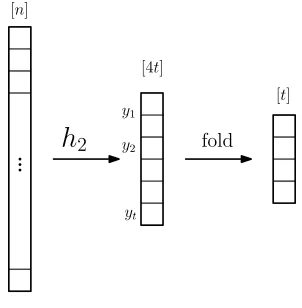
Step 4(Folding): We choose uniformly at randomI0⊆[4t]such that|I0|=t. We now fix an arbitrary map f :[4t]→[t]such that f is a bijection onI0and defineh(j):= f(h2(j)). The number of choices in

this step is the number of possibilities forI0which is 2O(t).

Since the number of possibilities for the random choices made in the above four steps, is bounded by 2O(t)nO(1), we see that|H_perfn,t |is at most 2O(t)nO(1).

y1

y2

yt [4t]

[t]

...

h

[n]

Figure 1: The basic framework of the perfect hash family construction.

We now show that a randomh∈Hn_perf,t has the properties stated in the lemma. Assumehis sampled as above. FixS⊆[n]such that|S|=t.

Fori∈[t], define the random variableXi=|h−₁1(i)∩S|and letX=∑i∈[t]Xi2. An easy computation

shows thatEh1[X]≤2t. LetE1denote the event thatX≤4t. By Markov’s inequality, Prh1[E1]≥1/2.

We condition on a choice ofh1so thatE1occurs.

We now analyze the second step. We say that eventE2holds if for eachi∈[t],yi=Xi2. We claim

that Pr[E2]≥1/2O(t). Since the number of random choices in Step 2 is only 2O(t), it suffices to argue that ∑i∈[t]Xi2≤4t. But this follows since we have conditioned onE1. We now condition on random choices

in Step 2 so thatE2occurs as well.

For the third step, giveni∈[t], we call the hash functionh_2,i collision-freeifh2,i is 1-1 on the set h−₁1(i)∩S. Sinceh2,i is chosen from a pairwise independent hash family, given any distinct j1,j2∈

h−₁1(i)∩S, the probability thath2,i(j1) =h2,i(j2)is 1/yi=1/Xi2. By a simple union bound, we can upper

bound the probability thath_2,iis not collision-free as follows:

Pr

h2,i

[h2,inot collision-free] =Pr h2,i

∃j16= j2∈h−11(i)∩S: h2,i(j1) =h2,i(j2)

≤

Xi

2

· 1 X2

i ≤1

2.

functions have been chosen using a suitable expander walk, byLemma 2.10, we see that

Pr[E3] = Pr

w∈_W(G1,...,Gt)

[∀i∈[t]: h₂,icollision-free]≥1/2O(t).

We condition on a choice for the hash functionsh2,1, . . . ,h2,t so thatE3also occurs. Note that given

h1andh2,ifori∈[t], the hash functionh2:[n]→[4t]is completely determined.

Moreover, conditioned on the eventsE1,E2,andE3, we claim thath2is 1-1 onS. To see this, consider

any distinct j₁,j₂∈S. Ifh₁(j₁)6=h₁(j₂), then we haveh₂(j₁)=6 h₂(j₂)straight away from (6.1). On the other hand, ifh1(j1) =h1(j2) =i, then from (6.1) we see that|h2(j1)−h2(j2)|=|h2,i(j1)−h2,i(j2)| 6=0,

where the last inequality follows from the fact thatE3holds and hence eachh2,iis collision-free. This

shows thath₂is 1-1 onS. LetI denote the seth₂(S)which is a subset of[4t]of size exactlyt. LetE4denote the event thatI0=I. The probability thatE4occurs is exactly 4tt

−1

=1/2O(t). When

E4 occurs as well, the function f maps I bijectively to[t]and hence the functionh= f◦h2 mapsS

bijectively to[t]as well, which is exactly what we want.

Thus the probability of sampling such a “good”his at least Pr[E1∧E2∧E3∧E4] =1/2O(t), which

proves the lemma.

The construction of the fractional perfect hash family is almost analogous to the construction of the perfect hash family above, though the details are somewhat more involved, as we have to ensure that each bucket in the hash has roughly equal weight.

Lemma2.13(restated). For anyn,t∈_Nsuch thatt≤n, there is an explicit family of hash functions

Hn,t

frac⊆[t][

n]_{of size 2}O(t)_nO(1)_{such that for anyz∈[0,1]}n_{such that}

∑j∈[n]zj≥10t, we have

Pr

h∈Hn_frac,t

"

∀i∈[t],0.01∑j∈[n]zj

t ≤_j∈h

∑

zj≤10

∑j∈[n]zj t

#

≥ 1

2O(t).

Proof. ForS⊆[n], we definez(S)to be∑j∈Szj. By assumption, we havez([n])≥10t. Without loss of

generality, we assume thatz([n]) =10t(otherwise, we work with ˜z= (10t/z([n]))zwhich satisfies this property; since we prove the lemma for ˜z, it is true forzas well). We thus need to constructHn_frac,t such that

Pr

h∈Hn_frac,t

∀i∈[t],z(h−1(i))∈[0.1,100]≥ 1

2O(t).

We describe the formal construction by describing how to sample a random elementhofHn_frac,t . To sample a randomh∈Hn_frac,t , we do the following:

Step 1(Top-level hashing): We choose a pairwise independent hash functionh1:[n]→[10t]by

choosing a random seed to generatorGt_2-wise,n . ByFact 2.7, this requiresO(logn+logt) =O(logn)bits.

Step 2 (Guessing bucket sizes): We choose at random a subset I0 ⊆[10t] of size exactlyt and

y1, . . . ,y10t∈Nso that∑iyi≤30t. It can be checked that the number of possibilities forI0andy1, . . . ,y10t

is only 2O(t).

Step 3(Second-level hashing): ByFact 2.7, for eachi∈[10t], we have an explicit pairwise inde-pendent family of hash functions mapping[n]to[yi]given byGyi,n

2-wise. We assume w.l.o.g. that each

maximum seed length among them). LetV ={0,1}s_{. UsingFact 2.9, fix a sequence(G}

1, . . . ,G10t)of

10tmany(2s_,D,

λ)-expanders on setV withD=O(1)andλ ≤1/100. Choosingw∈W(G1, . . . ,G10t)

uniformly at random, seth2,i:[n]→[yi]to beG_2-wiseyi,n (vi(w)). Defineh2:[n]→[30t]as follows:

h₂(j) =

_∑

i<h1(j),i6∈I0

yi

!

+h_2,h1(j)(j).

Given the random choices made in the previous steps, the functionh₂ is completely determined by

|W(G1, . . . ,G10t)|, which is 2O(t)·nO(1).

Step 4(Folding): This step is completely deterministic given the random choices made in the previous steps. We fix an arbitrary map f :(I0× {0})∪([10t]× {1})→[t]with the following properties: (a) f is 1-1 onI0× {0}, (b) f is 10-to-1 on[10t]× {1}. We now defineh:[n]→[t]. Defineh(j)as

h(j) = (

f(h₁(j),0) ifh₁(j)∈I0,

f(h2(j),1) otherwise.

It is easy to check that|H_fracn,t |, which is the number of possibilities for the random choices made in the above steps, is bounded by 2O(t)nO(1), exactly as required.

We now show that a randomh∈Hn_frac,t has the properties stated in the lemma. Assumehis sampled as above. We analyze the construction step-by-step. First, we recall the following easy consequence of the Paley-Zygmund inequality:

Fact 6.1. For any non-negative random variable Z we have

Pr[Z≥0.1E[Z]]≥0.9(E[

Z])2 E[Z2] .

Considerh1sampled in the first step. Define, for eachi∈[10t], the random variablesXi=z(h−₁1(i))

andYi=∑j16=j2:h1(j1)=h1(j2)=izj1zj2, and letX=∑i∈[10t]Xi2andY =∑i∈[10t]Yi. An easy calculation shows

thatX=∑j∈[n]z2j+Y ≤10t+Y. Hence,Eh1[X]≤10t+Eh1[Y]and moreover

E

h1

[Y] =

_∑

j16=j2

zj1zj2Pr

h1

[h1(j1) =h1(j2)]≤

z([n])2

10t =10t.

LetE1denote the event thatY ≤20t. By Markov’s inequality, this happens with probability at least 1/2.

We condition on any choice ofh1so thatE1occurs. Note that in this case, we haveX≤10t+Y ≤30t.

LetZ =Xi for a randomly chosen i∈[10t]. Clearly, we have Ei[Z] = (1/10t)∑iXi=1 and also

Ei[Z2] = (1/10t)∑iXi2 = (1/10t)X ≤3. Thus, Fact 6.1 implies that for random i∈[n], we have

Pri[Z≥0.1]≥0.3. Markov’s Inequality tells us that Pri[Z>10]≤0.1. Putting things together, we

see that if we setI ={i∈[10t]|Xi∈[0.1,10]}, then|I| ≥0.2×10t=2t. The elements of I will be referred to as themedium-sized buckets.

We now analyze the second step. We say that eventE2holds if (a)I0 containsonlymedium-sized

buckets, and (b) for eachi∈[10t],yi=dYie. We claim that Pr[E2]≥1/2O(t). Since the number of random