Article Title & Authors

(1)

Does The Effect of Trade on Growth Differentiate

for Countries with Different Income Levels? New

Panel Evidence

Aslı Seda Kurt

Assist. Prof. Dr., Dokuz Eylul University, Faculty of Economics and Administrative Sciences, Department of Economics, Dokuzcesmeler Campus, 35160, Buca, Izmir, Turkey

Utku Utkulu

Prof. Dr., Dokuz Eylul University, Faculty of Economics and Administrative Sciences, Department of Economics, Dokuzcesmeler Campus, 35160, Buca, Izmir, Turkey

Abstract

The effects of trade on growth have been one of the most popular issues in economic literature. Though there is a vast number of a theoretical and empirical study concerning the topic, there is still an ongoing debate over to what extent and in which direction growth is affected by trade. The main purpose of this paper is to obtain comprehensive empirical findings and find out whether trade has a significant effect on growth and also whether this effect differentiates for countries with different income levels. The direction, degree and power of the effects of trade on growth are investigated by considering exports, imports and trade volume. Since we have taken into consideration the fact that this effect may differ in countries of different income levels, we have adopted a classification of countries suggested by the World Bank depending on income levels of the countries, and an annual data set comprising the period between 1995 and 2015 is used for the selected countries. Panel data analysis is conducted and more specifically, common correlated effects initially introduced by Pesaran (2006), and panel autoregressive distributed lag models put forward by Pesaran, Shin and Smith (1999) are estimated since the series have both cross-sectional and time series properties. Empirical findings suggest that trade affects national income positively. We have strong evidence that trade leads to growth mainly in high income countries. Besides, country specific estimates are also presented unlike the literature.

Keywords: Trade, growth, common correlated effects estimator, panel autoregressive distributed lag models. JEL Classification Codes: C33, F140, O40.

1.INTRODUCTION

In the light of classical and neoclassical theories of trade, countries liberalize their economic policies including their trade policies. On the empirical side, however, it is still not clear-cut whether free trade affects growth positively. This paper aims to explore the relationship between trade and growth by performing a multi-country analysis and using a large sample.

Theories concerning the relationship between trade and wealth date back to A. Smith and D. Ricardo. These classical theories of trade claim that trade increases the wealth of nations. In other words, possible wealth-increasing effects of trade make it reasonable for the nations to trade and follow liberal policies. According to macroeconomics, free trade is advantageous for the nations as long as it enables the economy to growth.

Early neoclassical growth models, such as Solow (1956) imply that trade policies have no effect on growth due to the fact that technological change is assumed to be exogenous in these models. Advanced growth models developed by Romer (1986), Lucas (1988) and Barro (1991) state that technological change is assumed to be endogenous which makes it possible to model the long run growth effects of trade. Recent contributions to the area of trade, technology and growth are as follows: Grossman and Helpman (1989a, 1989b, 1990, 1991a, 1991b, 1991c).

Theories concerning the relationship between trade and growth can be evaluated in two perspectives: in terms of macroeconomics and in the light of trade theories (Gandolfo; 1998). Direction of the causality between trade and growth is generally from the first to the latter in the macroeconomic theory. Keynesian multiplier, twin deficits hypothesis, export-led growth models, and theories with regard to the relationship between growth and balance of payments are good examples for the abovementioned causality. On the contrary, the direction of the relationship between trade and growth in the theories of trade is just the opposite of the macroeconomic theory. Hicks (1953), Johnson (1955), Rybczynski (1956) and Bhagwati (The Theory of Immiserizing Growth) (1958) claim that trade is affected by growth. We follow the first in this paper.

(2)

countries an opportunity to benefit each other’s factors of production. One can easily understand that exports affects total output because of several reasons. Exports allows countries to specialize based on comparative advantages, and so ensures more efficient resource allocation in the economy. Besides, exports enables economies to benefit economies of scale and promotes technological development. All these arguments put forward that there is a strong relationship between exports and growth. On the other hand, when capital shortfall and dependency on foreign-source (raw materials, intermediate goods, energy etc.) of the countries (especially underdeveloped and developing countries) are taken into account, it can be seen that there is also a strong relationship between imports and growth. Otherwise, trade volume is a widely used indicator for trade to reveal the effect of trade on growth. Another important channel through which trade affect growth positively is knowledge and technology transfers. So, exports, imports and trade volume have been used as the indicators for trade in this paper.

The organization of the paper is as follows: In the second section, empirical literature is summarized. Data and the model are introduced in the second section. In the third section, empirical methodology is given. The following section presents the findings. And finally the conclusions and implications are discussed.

2. EMPIRICAL LITERATURE

There are many empirical studies in the field. Most of the papers find that trade has a positive effect on growth. Greenaway and Sapsford (1993) applied Granger-Sims causality and found that the direction of the causality is from terms of trade to trade policy. Ghatak, Milner and Utkulu (1995) carried out cointegration analysis and showed that there was a stable long run relationship between trade liberalization and per-capita gross domestic product (GDP) in Turkey. Ghatak and Utkulu (1996) applied cointegration analysis and according to their findings, trade liberalization affected growth both in the short and long run in Turkey, Malaysia and India. In another paper, Ghatak, Milner and Utkulu (1997) adopted cointegration and causality tests. To their findings, there was an export-led growth in Malaysia for the period 1955-1990. One another paper for trade and growth was carried out by Utkulu and Özdemir (2005). In this paper, the researchers performed causality analysis and to their findings, trade policy was of great importance for growth both in the short and long run. Probit models were used by Cavallo and Frankel (2007) in order to search the effects of trade. They showed that trade enabled the economy to be less sensitive to external shocks. Matedeen, Matedeen and Seetanah (2011) investigated the effect of trade on growth in Mauritius by following vector error correction mechanism (VECM) framework. They concluded that trade is an engine of growth as accepted in the literature. So, the vast of the literature supports that there is a positive effect of trade on growth.

(3)

3. THE MODEL AND DATA

Trade theories do not generally present an empirical framework while the relationship between trade and growth is examined via simplex models in macroeconomics. Export led growth models are mostly used in the empirical literature. However, it is of great significance for indicators for trade to take into account. That’s why standard exports and imports models are not referred in this paper. New theoretical models are needed to analyze the interaction between trade and growth. But, there are several problems in developing new models. For example, Obstfeld and Rogoff (1996) use variables of financial account that are expected to be equivalent to that of current account theoretically because of the difficulties in modeling (Obstfeld and Rogoff, 1996: 15). When the models developed in the 2000s are taken into consideration, it is seen that assumption of one good has been adopted for simplicity (Benge and Wells, 2002; Pacho, 2008). In fact, there must be at least two goods for trade to start. Nevertheless, it is really difficult for the models with two goods to be solved because such models have to include relative prices and real exchange rates. Under these limitations, the models based on production function developed by Balassa (1978), Tyler (1981) and Ram (1985) have been adopted in this paper. In this context, production function can be rewritten as follows:

, , (1)

In equation (1) represents the amount of capital, represents the amount of labor and represents trade. If total differentiation of equation (1) is taken and the equation is written in growth form, equation (2) is obtained:

. . . (2)

Equation (2) can be manipulated as follows: /

/ .

/ / .

/

/ . (3)

While is a constant term, /_/ , /_/ and /_/ , equation (3) can be rewritten as follows:

(4)

Here and represent marginal physical product of capital and labor respectively while shows the effect of trade on growth. The variables are used in empirical analysis in the light of this model as follows:

: Growth rate of real GDP (%),

: Growth rate of gross fixed capital formation (%), : Growth rate of labor force (%),

: Growth rate of exports/imports/trade volume (%)

The models have been named according to the trade indicator used in the model. So there are three models: exports model, imports model and trade volume model. All variables are used as growth rates and in real terms.

Annual data from 1995 to 2015 is used and all data is gathered from the database of World Bank (World Development Indicators) and International Labour Organization (ILO). The countries covered in the analysis are shown in Table 2. The countries are selected depending on the data availability, and classified depending on World Bank’s classification.

Table 1: Countries and Data Range

Countries Data Range High Income Countries (HI): Australia, Austria, Belgium, Canada, Chile,

Czech Republic, Denmark, France, Germany, Greece, Hong Kong, Ireland, Luxembourg, Macao, The Netherlands, Norway, Poland, Portugal, Slovak Republic, Spain, Sweden, Switzerland, Trinidad and Tobago, The United Kingdom, The United States.

1995-2015

Upper Middle Income Countries (UMI): Belarus, Brazil, Bulgaria,

Dominican Republic, Macedonia, Malaysia, Mexico, Paraguay, Romania,

Russian Federation, Turkey. 1995-2015

Lower Middle Income Countries (LMI): Arab Republic of Egypt, Indonesia,

Moldova, Morocco, Philippines, Ukraine, Vietnam, Sri Lanka. 1995-2015

Low Income Countries (LI): Benin, Burkina Faso, Congo Democratic Republic, Madagascar, Mali, Mozambique, Rwanda, Senegal, Sierra Leone, Tanzania, Uganda.

(4)

4. EMPIRICAL METHODOLOGY

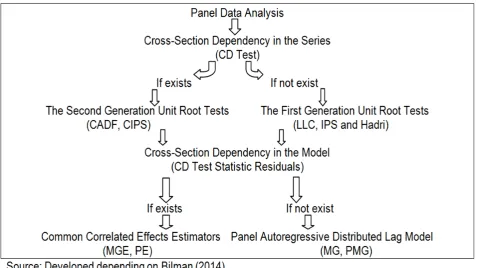
In this paper, we apply panel data analysis which combines time series and cross-section data as introduced by Baltagi (2002). Pesaran (2004) puts forward that cross-section dependency must be taken into consideration in panel data. Cross-section dependency is the case when a shock to a specific country affects other countries as well. Figure 1 sums up the empirical methodology adopted in this paper.

Figure 1: Econometric Methodology

If there is a cross-section dependency in the series, the second generation unit root tests would lead to reliable results. If there is cross-section independency, the results of the first generation unit root tests would be reliable. As for unit root tests, Levin, Lin and Chu (LLC) (2002) assumes that the coefficient of the lagged values of the dependent variable is homogenous for all cross-section units while Im, Pesaran and Shin (IPS) (2003) assumes that the aforesaid coefficient is heterogeneous. The null hypothesis in this testing procedures are generally formulated as unit root/non-stationarity while Hadri (2000)’s approach adopts the null of no unit root/stationarity. Pesaran (2007) suggests a panel unit root test considering cross-section dependency named cross-sectionally augmented Dickey-Fuller (CADF). Cross-sectionally Im, Pesaran and Shin statistics (CIPS) is calculated as the average of CADF.

Pesaran (2004) also suggests two estimators named Mean Group Estimators (MGE) and Pooled Estimators (PE) which take into account cross-section dependency. MGE are calculated as the arithmetic average of the long-run coefficients of each cross-section units. In pooled estimators, long-run parameters are assumed to be the same. This estimator is more efficient in small samples. These two estimators are called common correlated effects estimators (CCE) and these estimators are more efficient and consistent even when the series are not stationary. Holly and Raissi (2009) and Nazlıoğlu (2010) stated that CCE estimators would lead to reliable results even when the series are stationary, difference stationary and cointegrated by referring Pesaran (2006) and Kapetanios, Pesaran and Yamagata (2009).

(5)

5. FINDINGS

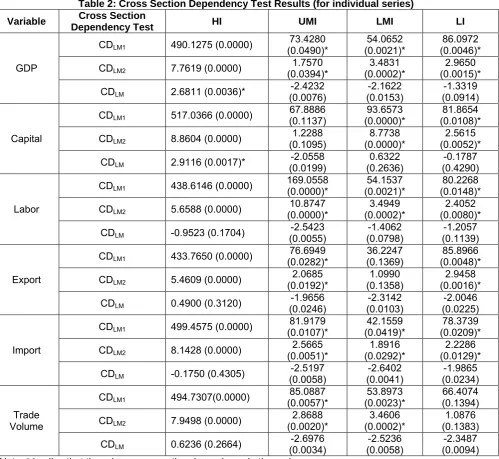
Time series properties of the series are tested by panel unit root tests. As explained before, if there is cross-section dependency in the series, the second generation unit root tests would lead to reliable results and vice versa. So, cross section dependency should be examined firstly. Table 2 summarizes the results. Only in high income country group (HI), the number of cross sections is greater than time units, and so CDLM test results are taken into consideration for this group. To the results, there is a cross section dependency in GDP and capital in high income country group. For other country groups (in which the number of cross sections are lower than the length of time series), CDLM1 and CDLM2 tests results are considered. There is no cross section

dependency in the series of capital, exports and trade volume in upper middle income countries (UMI), lower middle income countries (LMI) and low income countries (LI) respectively.

Table 2: Cross Section Dependency Test Results (for individual series)

Variable Cross Section

Dependency Test HI UMI LMI LI

GDP

CDLM1 490.1275 (0.0000) _(0.0490)*73.4280 _(0.0021)*54.0652 _(0.0046)*86.0972

CDLM2 7.7619 (0.0000) _(0.0394)*1.7570 _(0.0002)*3.4831 _(0.0015)*2.9650

CDLM 2.6811 (0.0036)* _(0.0076)-2.4232 _(0.0153)-2.1622 _(0.0914)-1.3319

Capital

CDLM1 517.0366 (0.0000) _(0.1137)67.8886 _(0.0000)*93.6573 _(0.0108)*81.8654

CDLM2 8.8604 (0.0000) _(0.1095)1.2288 _(0.0000)*8.7738 _(0.0052)*2.5615

CDLM 2.9116 (0.0017)* _(0.0199)-2.0558 _(0.2636)0.6322 _(0.4290)-0.1787

Labor

CDLM1 438.6146 (0.0000) 169.0558 _(0.0000)* _(0.0021)*54.1537 _(0.0148)*80.2268

CDLM2 5.6588 (0.0000) _(0.0000)*10.8747 _(0.0002)*3.4949 _(0.0080)*2.4052

CDLM -0.9523 (0.1704) _(0.0055)-2.5423 _(0.0798)-1.4062 _(0.1139)-1.2057

Export

CDLM1 433.7650 (0.0000) _(0.0282)*76.6949 _(0.1369)36.2247 _(0.0048)*85.8966

CDLM2 5.4609 (0.0000) _(0.0192)*2.0685 _(0.1358)1.0990 _(0.0016)*2.9458

CDLM 0.4900 (0.3120) _(0.0246)-1.9656 _(0.0103)-2.3142 _(0.0225)-2.0046

Import

CDLM1 499.4575 (0.0000) _(0.0107)*81.9179 _(0.0419)*42.1559 _(0.0209)*78.3739

CDLM2 8.1428 (0.0000) _(0.0051)*2.5665 _(0.0292)*1.8916 _(0.0129)*2.2286

CDLM -0.1750 (0.4305) _(0.0058)-2.5197 _(0.0041)-2.6402 _(0.0234)-1.9865

Trade Volume

CDLM1 494.7307(0.0000) _(0.0057)*85.0887 _(0.0023)*53.8973 66.4074 _(0.1394)

CDLM2 7.9498 (0.0000) _(0.0020)*2.8688 _(0.0002)*3.4606 _(0.1383)1.0876

CDLM 0.6236 (0.2664) _(0.0034)-2.6976 _(0.0058)-2.5236 _(0.0094)-2.3487

Note: * implies that there is a cross section dependency in the series.

(6)

Table 3: Unit Root Test Results

Variable Unit Root Test HI UMI LMI LI

GDP

LLC -12.1087 (0.0000)* -5.81134 (0.0000)* -1.65806 (0.0487)* -8.87852 (0.0000)* IPS -6.54435 (0.0000)* -6.89720 (0.0000)* -4.76214 (0.0000)* -9.60202 (0.0000)* Hadri 13.9868 (0.0000) -0.13570 (0.5540)* 1.00033 (0.1586)* 5.39365 (0.0000) CIPS -2.0523 [-2.21] -2.7686 [-2.34]* -2.9311 [-2.34]* -2.6285 [-2.34]*

Capital

LLC -19.3700 (0.0000)* -8.46238 (0.0000)* -4.63747 (0.0000)* -17.4326 (0.0000)* IPS -14.5652 (0.0000)* -7.84762 (0.0000)* -4.60548 (0.0000)* -13.7458 (0.0000)* Hadri 3.04915 (0.0011) 0.32340 (0.3732)* 1.89546 (0.0290) -0.30732 (0.6207)* CIPS -2.6818 [-2.21]* -2.7659 [-2.34]* -2.1796 [-2.34] -2.7726 [-2.34]*

Labor

LLC -4.21261 (0.0000)* -0.59566 (0.2757) -1.24231 (0.1071) -0.89371 (0.1857) IPS -5.86487 (0.0000)* -3.33180 (0.0004)* -3.11308 (0.0009)* -3.11831 (0.0009)* Hadri 5.31741 (0.0000) 2.54747 (0.0054) 1.76985 (0.0384) 1.17520 (0.1200)* CIPS -2.3603 [-2.21]* -1.9235 [-2.34] -2.4034 [-2.34]* -1.9844 [-2.34]

Export

LLC -10.6794 (0.0000)* -11.3856 (0.0000)* -9.96733 (0.0000)* -11.6015 (0.0000)* IPS -7.94757 (0.0000)* -10.0903 (0.0000)* -8.99272 (0.0000)* -10.1397 (0.0000)* Hadri 4.37829 (0.0000) 0.85239 (0.1970)* 1.58503 (0.0565)* 2.45783 (0.0070) CIPS -2.6853 [-2.21]* -2.7711 [-2.34]* -2.3817 [-2.34]* -3.5457 [-2.34]*

Import

LLC -15.2335 (0.0000)* -12.7361 (0.0000)* -9.63267 (0.0000)* -12.8609 (0.0000)* IPS -12.6709 (0.0000)* -11.3022 (0.0000)* -8.04647 (0.0000)* -12.9623 (0.0000)* Hadri 5.20452 (0.0000) 0.69676 (0.2430)* 0.52295 (0.3005)* 1.60594 (0.0541)* CIPS -2.5219 [-2.21]* -2.8404 [-2.34]* -2.4948 [-2.34]* -3.3145 [-2.34]*

Trade Volume

LLC -15.3550 (0.0000)* -12.1343 (0.0000)* -9.38447 (0.0000)* -10.2136 (0.0000)* IPS -12.5979 (0.0000)* -10.2453 (0.0000)* -8.04377 (0.0000)* -10.4761 (0.0000)* Hadri 5.59321 (0.0000) 1.73346 (0.0415)* 0.87401 (0.1911)* 1.26269 (0.1033)* CIPS -2.4730 [-2.21]* -2.8540 [-2.34]* -2.9540 [-2.34]* -2.4729 [-2.34]* Note: (a) The optimal lag length has been chosen according to Schwarz information criteria, Bartlett Kernel method and bandwith has been identified in accordance with Newey-West methodology. (b) For CIPS, numbers in brackets denote critical values suggested by Pesaran (2007). For other unit root tests, numbers in parentheses denote probabilities.

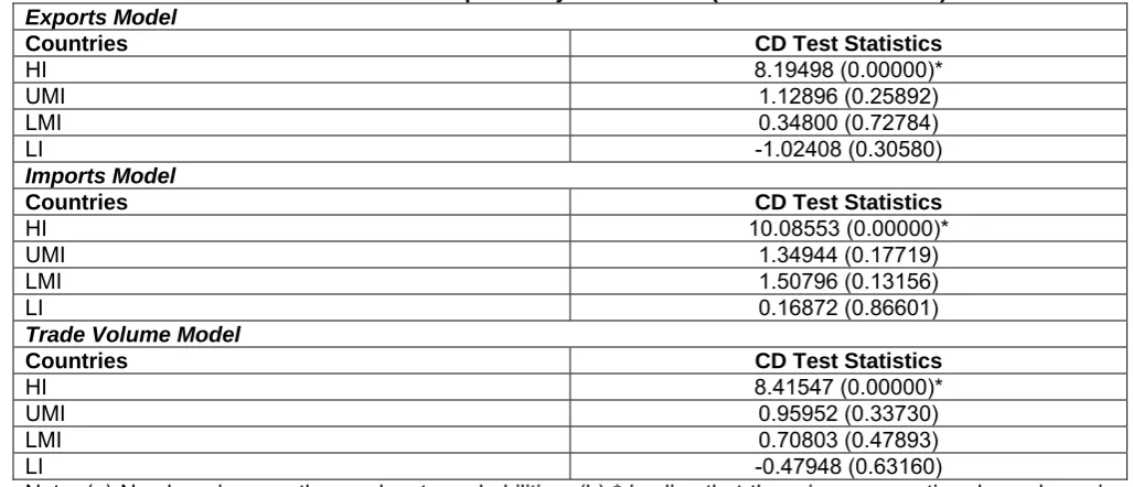
In this paper, long run coefficients are estimated by adopting CCE. This methodology considers cross section dependency and allows heterogeneity in panel data. To the Table 4, there is cross section dependency only for HI group in all models.

Table 4: Cross Section Dependency Test Results (for individual models)

Exports Model

Countries CD Test Statistics

HI 8.19498 (0.00000)*

UMI 1.12896 (0.25892)

LMI 0.34800 (0.72784)

LI -1.02408 (0.30580)

Imports Model

HI 10.08553 (0.00000)*

UMI 1.34944 (0.17719)

LMI 1.50796 (0.13156)

LI 0.16872 (0.86601)

Trade Volume Model

HI 8.41547 (0.00000)*

UMI 0.95952 (0.33730)

LMI 0.70803 (0.47893)

LI -0.47948 (0.63160)

(7)

For the models in which there is cross section dependency, CCE results are summarized in Table 5, 6, and 7. In HI, exports is the main source of growth and capital is also an important determinant of growth. The coefficient of labor is not statistically significant.

Table 5: Pesaran (2006) CCE Results for Exports Model HI

Pesaran (2006) CCE (Mean Group Estimator)

Variables Coefficients and t-Statistics

Capital 0.1562 (8.6815)***

Labor 0.1067 (1.2420)

Exports 0.1881 (5.4383)***

Pesaran (2006) CCE (Pooled Estimator)

Capital 0.1495 (7.7247)***

Labor 0.1066 (0.6824)

Exports 0.2660 (5.0055)***

Note: (a) Newey-West variance-covariance estimator has been considered in pooled estimators. (b) Numbers in parentheses denote t-statistics. (c) ***, **, * imply the significance at 1%, 5% and 10% levels respectively.

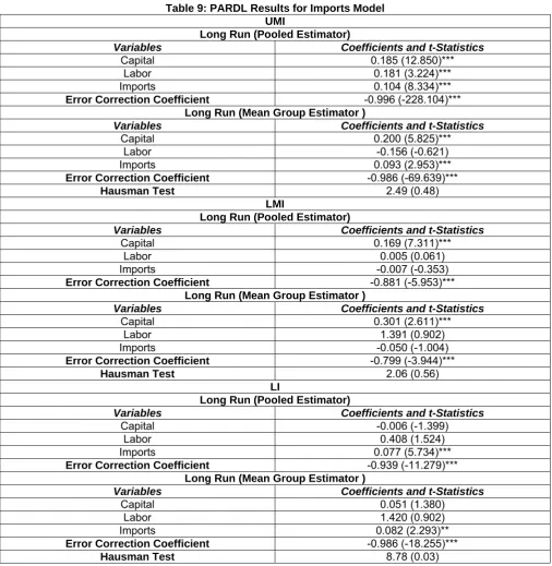
In imports models, it is readily seen that imports affects growth positively in HI. On the other hand, when imports model is considered, capital accumulation has a leading role in stimulating growth in HI group.

Table 6: Pesaran (2006) CCE Results for Imports Model HI

Capital 0.1409 (5.9261)***

Labor 0.0866 (1.0236)

Imports 0.0949 (3.1994)***

Capital 0.1192 (3.6199)***

Labor -0.0226 (-0.1076)

Imports 0.1384 (3.3238)***

Note: (a) Newey-West variance-covariance estimator has been considered in pooled estimators. (b) Numbers in parentheses denote t-statistics. (c) ***, **, * imply the significance 1%, 5% and 10% levels respectively.

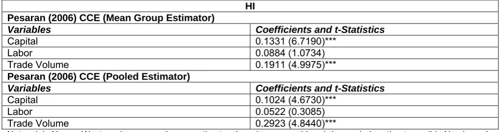
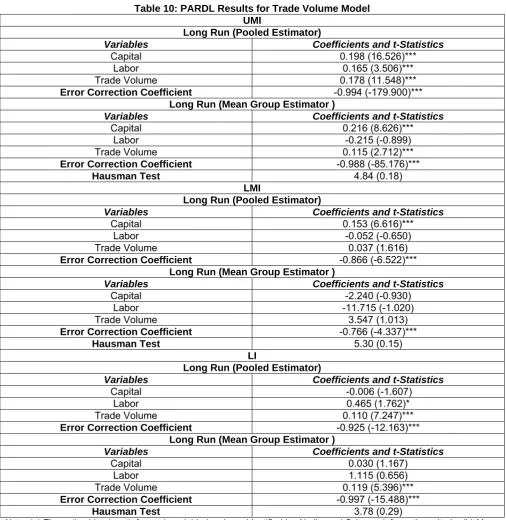
CCE results for trade volume model in HI group are presented in Table 7. To the findings, trade volume has a statistically significant, positive and the strongest effect on growth in HI group. The results also imply that capital is another important variable stimulating the growth.

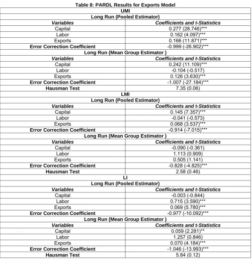
For the models where there is cross section independency, PARDL results are shown in Table 8, 9, and 10. When PARDL results for each three models are taken into consideration, it can be easily seen that error correction mechanism works. It means that there is a long run cointegration relationship among the variables involved in the models. Only in imports model for LI, mean group estimators are more efficient in accordance with Hausman test. As for the results of exports model for UMI group, all coefficients are statistically significant and have positive effect on growth. On the other hand, capital is the main driver of long run growth.

Table 7: Pesaran (2006) CCE Results for Trade Volume Model HI

Capital 0.1331 (6.7190)***

Labor 0.0884 (1.0734)

Trade Volume 0.1911 (4.9975)***

Capital 0.1024 (4.6730)***

Labor 0.0522 (0.3085)

Trade Volume 0.2923 (4.8440)***

(8)

Table 8 shows that pooled estimators are more efficient in LMI group according to the Hausman test. To the findings, capital and exports have a statistically significant and positive effect on growth. As for LI group, only labor and exports have a statistically significant and positive effect on growth.

Table 8: PARDL Results for Exports Model UMI

Long Run (Pooled Estimator)

Capital 0.277 (28.746)***

Labor 0.162 (4.097)***

Exports 0.166 (11.871)***

Error Correction Coefficient -0.999 (-26.902)*** Long Run (Mean Group Estimator )

Capital 0.242 (11.109)***

Labor -0.104 (-0.517)

Exports 0.126 (3.630)***

Error Correction Coefficient -1.007 (-27.184)*** Hausman Test 7.35 (0.06)

LMI

Capital 0.145 (7.357)***

Labor -0.041 (-0.573)

Exports 0.068 (3.537)***

Capital -0.090 (-0.361)

Labor 1.113 (0.909)

Exports 0.505 (1.141)

LI

Capital -0.003 (-0.844)

Labor 0.715 (3.590)***

Exports 0.069 (5.780)***

Capital 0.059 (2.281)**

Labor 1.257 (0.846)

Exports 0.070 (4.184)***

Note: (a) The optimal lag length for each variable has been identified by Akaike and Schwarz information criteria. (b) Mean group estimators are used as the initials in the estimation of the pooled maximum likelihood function. (c) Numbers in parentheses denote t-statistics. (d) ***, **, * imply the significance 1%, 5% and 10% levels respectively. (e) Numbers in parentheses denote possibilities for Hausman test statistics.

(9)

Table 9: PARDL Results for Imports Model UMI

Capital 0.185 (12.850)***

Labor 0.181 (3.224)***

Imports 0.104 (8.334)***

Capital 0.200 (5.825)***

Labor -0.156 (-0.621)

Imports 0.093 (2.953)***

LMI

Capital 0.169 (7.311)***

Labor 0.005 (0.061)

Imports -0.007 (-0.353)

Capital 0.301 (2.611)***

Labor 1.391 (0.902)

Imports -0.050 (-1.004)

LI

Capital -0.006 (-1.399)

Labor 0.408 (1.524)

Imports 0.077 (5.734)***

Capital 0.051 (1.380)

Labor 1.420 (0.902)

Imports 0.082 (2.293)**

(10)

Table 10: PARDL Results for Trade Volume Model UMI

Capital 0.198 (16.526)***

Labor 0.165 (3.506)***

Trade Volume 0.178 (11.548)***

Capital 0.216 (8.626)***

Labor -0.215 (-0.899)

Trade Volume 0.115 (2.712)***

LMI

Capital 0.153 (6.616)***

Labor -0.052 (-0.650)

Trade Volume 0.037 (1.616)

Capital -2.240 (-0.930)

Labor -11.715 (-1.020)

Trade Volume 3.547 (1.013)

LI

Capital -0.006 (-1.607)

Labor 0.465 (1.762)*

Trade Volume 0.110 (7.247)***

Capital 0.030 (1.167)

Labor 1.115 (0.656)

Trade Volume 0.119 (5.396)***

(11)

6. CONCLUSION

This paper analyzes the role of trade on growth. The paper also emphasizes the role of other factors (capital and labor as basic factors of production) affecting growth. The results of the paper support positive effect of trade on growth. In other words, liberal trade policy applications have a positive effect on growth.

As a measure for trade, growth rate of exports and imports of goods and services, and trade volume are taken into consideration. Based on the findings of the paper, increase in trade affects growth positively in the countries from different income levels over the period 1995-2015. 1995 is chosen as a start date because World Trade Organization (WTO) of which the main aim is to liberalize the world trade has been established in this year.

Panel data analyses have been adopted to explore the long run effects of trade on growth. Unlike the other many papers in the related literature, country specific estimations are also reported in this paper. Thus, the difference between the results for groups and countries can be seen, and this paper also presents wider empirical evidence.

There is cross section dependency only in high income group. It may originate from the fact that commercial and financial flows are greater among these countries. In high income countries of which the share in the world trade is very high, trade can be seen as the engine of the growth in accordance with the findings of this paper. An important characteristic of these countries is that the economy works with high capacity. So, the growth rates of gross fixed capital and labor force have a limited effect on growth in these countries. Moreover, growth rate of labor force has a negative effect in some countries when country specific results are considered (for example in Australia, Chile and Czech Republic). Only in imports model, capital has the variable of which effect is the strongest on growth. Another remarkable point is that imports has a negative effect on growth in only Germany. Generally, high income countries produce new products via new knowledge and technology and sell them around the world. In other words, trade (especially exports) determines the growth performance.

As always stated in the growth literature, capital accumulation is very important in terms of growth. Conveniently, the findings imply that growth in gross fixed capital plays a leading role in upper middle income and lower middle income countries. The main drivers are capital and labor in upper middle income countries in which capacity utilization rate is growing. Nevertheless, trade is also of great importance in stimulating growth. These countries in development process increase their production capacity firstly, and then sell goods both in domestic market and foreign markets. In lower middle income countries, growth rate of capital is seen as the main determinant of growth. Trade (especially exports) is also an important driver of the growth. As for the country specific results, exports model works in only four countries in accordance with the error correction mechanism: Bulgaria, Mexico, Russian Federation and Turkey. To these results, growth of fixed capital has the strongest effect on growth. Exports is the second and labor is the third. Only in Turkey, error correction mechanism works in imports and trade volume models. And not surprisingly, findings support that capital accumulation is the key factor to growth. Similarly, growth of fixed capital has the stronger effect on growth in lower middle income countries when country specific estimations are considered. The exports model works in Arab Republic of Egypt, Morocco, Philippines, Ukraine and Vietnam considering the error correction coefficient. The imports model works in Morocco, Philippines and Vietnam while trade volume model works in Arab Republic of Egypt, Moldova, Morocco, Philippines, Ukraine and Vietnam.

In low income countries, labor has a leading determinant of growth. The distinguishing feature of these countries is that labor intensive goods are produced and sell around the world. Increasing amount of labor force is more educated, and so the rise in the labor force promotes growth in these countries. Besides these countries need foreign sources to produce and sell, so imports is also an important driver of growth. When country specific estimates are taken into consideration, growth of labor force has the strongest effect on growth once again. The exports model works in Burkina Faso and Congo, Democratic Republic. The imports and trade volume models work only in Congo, Democratic Republic and Rwanda.

Consequently, it is found that trade is good for growth in line with the theory. It may be interesting that different measures of trade are considered and new mathematical models of open economy with multiproduct are developed in further researches.

ACKNOWLEDGEMENTS

(12)

REFERENCES

Balassa, B. (1978). Exports and Economic Growth: Further Evidence. Journal of Development Economics, 5: 181-189.

Baltagi, B. H. (2002). Recent Developments in the Econometrics of Panel Data Volumes I and II, Cheltenham: Edward Elgar Publishing.

Barro, R. (1991). Economic Growth in a Cross-Section of Countries. Quarterly Journal of Economics, 106 (2): 407-443.

Benge, M. and Wells, G. (2002). Growth and the Current Account in a Small Open Economy. The Journal of Economic Education. 33 (2): 152-165.

Bhagwati, J. (1958). Immiserizing Growth: A Geometrical Note. The Review of Economic Studies, 25 (3): 201-205.

Bilman, A. S. (2014). Ticari Açıklık Büyüme Etkileşimi: Panel Veri Analizi ve Ülkelerarası Karşılaştırma. Unpublished PhD. Izmir: Dokuz Eylul University Graduate School of Social Sciences.

Buch, C. M. and Toubal, F. (2009). Openness and Growth: The Long Shadow of the Berlin Wall. Journal of Macroeconomics, 31: 409-422.

Cavallo, E. and Frankel, J.A. (2007). Does Openness to Trade Make Countries More Vulnerable to Sudden Stops, or Less? Using Gravity to Establish Causality. Inter-America Development Bank Research Dpartment Working Paper #618.

Chang, R. Kaltani, L. and Loayza, N. (2009). Openness Can Be Good for Growth: The Role of Policy Complementaries. Journal of Development Economics, 90: 33-49.

Chen, P. and Gupta, R. (2006). An Investigation of Openness and Economic Growth Using Panel Estimation, http://www.up.ac.za/up/web/en/academic/economics/index.html. (15.03.2011).

Dritsakis, N. and P. Stamatiou. (2016). Trade Openness and Economic Growth: A Panel Cointegration and Causality Analysis for the Newest EU Countries. The Romanian Economic Journal, 59, 45-60. Fetahi-Vehabi, M., Sadiku, L. and M. Petkovski. (2015). Empirical Analysis of the Effects of Trade Openness on

Economic Growth: An Evidence for South East European Countries. Procedia Economics and Finance, 19 (2015), 17-26.

Gandolfo, G. (1998). International Trade Theory and Policy. Springer.

Ghatak, S., Milner, C. and Utkulu, U. (1995). Trade Liberalization and Endogenous Growth: Some Evidence for Turkey. Economics of Planning, 28: 147 – 167.

Ghatak, S. and Utkulu, U. (1996). Trade Liberalization and Economic Development: The Asian Experience: Turkey, Malaysia and India. Trade and Development: Essays in Honour of Jagdish Bhagwati. (pp. 81-116). Editors: V.N. Balasubramanyam and D. Greenaway. England, Macmillan Publication. Ghatak, S., Milner, C. and Utkulu, U. (1997). Exports, Export Composition and Growth: Cointegration and

Causality Evidence for Malaysia. Applied Economics, 29: 213-223.

Greenaway, D. and Sapsford, D. (1993). Liberalisation and the Terms of Trade in Turkey: A Causal Analysis. CREDIT Research Paper, No: 93/3.

Greenaway, D., Morgan, W. and Wright, P. (2002). Trade Liberalisation and Growth in Developing Countries. Journal of Development Economics, 67: 229-244.

Grossman, G. M. and Helpman, E. (1989a). Growth and Welfare in a Small Open Economy. NBER Working Paper Series, No. 2970.

Grossman, G. M. and Helpman, E. (1989b). Product Development and International Trade. The Journal of Political Economy, 97 (6): 1261-1283.

Grossman, G. M. and Helpman, E. (1990). Comparative Advantage and Long-Run Growth. The American Economic Review, 80 (4): 796-815.

Grossman, G. M. and Helpman, E. (1991a). Quality Ladders in the Theory of Growth. The Review of Economic Studies, 58 (1): 43- 61.

Grossman, G. M. and Helpman, E. (1991b). Endogenous Product Cycles. The Economic Journal, 101 (408): 1214-1229.

Grossman, G. M. and Helpman, E. (1991c). Trade, Knowledge Spillowers and Growth. European Economic Review, 35: 517-526.

Hadri, K. (2000). Testing for Stationarity in Hetereogenous Panel Data. Econometrics Journal, 3, 148-161. Harrison, A. (1996). Openness and Growth: A Time-Series, Cross – Country analysis for Developing Countries.

(13)

Hicks, J. R. (1953). An Inaugural Lecture. Oxford Economic Papers, New Series, 5 (2): 117-135.

Holly, S. and Raissi, M. (2009). The Macroeconomic Effects of European Financial Development: a

Heterogeneous Panel Analysis. http://www.diw.de/documents/ publikationen/73/diw_01.c.96141.de/diw_finess_01040. pdf. (23.01.2014).

Im, K.S., Pesaran, M.H. and Shin, Y. (2003). Testing for Unit Roots in Heterogeneous Panels. Journal of Econometrics, 115, 53-74.

Jadoon, A. K., Rashid, H. A. and A. Azeem. (2015), “Trade Liberalization, Human Capital and Economic Growth: Empirical Evidence from Selected Asian Countries”, Pakistan Economic and Social Review, 53 (1), 113-132.

Johnson, H. G. (1955). Economic Expansion and International Trade. The Manchester School, 23 (2): 95-112. Kapetanios, G., Pesaran, M. H. and T. Yamagata. (2009). Panels with Nonstationary Multifactor Error

Structures. http://www.econ.cam.ac.uk/people/emeritus/mhp1b/wp09/ KPY _CCEunit_130609.pdf, (17.08.2016).

Kose, M.A., Prasad, E.S. and Terrones, M.E. (2006). How Do Trade and Financial Integration Affect the Relationship Between Growth and Volatility?. Journal of International Economics, 69: 176-202. Lee, H.Y., Ricci, L.A. and Rigobon, R. (2004). Once Again, Is Openness Good for Growth?. Journal of

Development Economics, 75: 451-472.

Levin, A., Lin, C.F. and Chu, C. (2002). Unit Root Test in Panel Data: Asymptotic and Finite Sample Properties. Journal of Econometrics, 108, 1–25.

Lucas, R. (1988). On The Mechanics of Economic Development. Journal of Monetary Economics, 22: 3-42. Matadeen, J., Matadeen, J. S. and B. Seetanah. (2011), “Trade Openness and Economic Growth: Evidence

from Mauritius”, http://sites.uom.ac.mu/wtochair/Conference%20 Proceedings/2.pdf, (16.08.2016). Nazlıoğlu, S. (2010). Makro İktisat Politikalarının Tarım Sektörü Üzerindeki Etkileri: Gelişmiş ve Gelişmekte

Olan Ülkeler İçin Bir Karşılaştırma. Unpublished PhD Thesis. Kayseri: Erciyes University Graduate School of Social Sciences.

Obstfeld, M. and Rogoff, K. (1996). Foundations of International Macroeconomics, Cambridge: The MIT Press. Pacho, W. (2008). The Solow Model in an Open Economy. papers.ssrn.com/sol3/

papers.cfm?abstract_id=1486671 . (08.11.2013).

Pesaran, M. H., Shin, Y. and Smith, R. P. (1999). Pooled Mean Group Estimation of Dynamic Heterogeneous Panels. Journal of the American Statistical Association, 94 (446): 621-624.

Pesaran, M. H. (2004). General Diagnostic Tests for Cross Section Dependence in Panels, CESifo Working Papers, No. 1229.

Pesaran, M. H. (2006). Estimation and Inference in Large Heterogeneous Panels with a Multifactor Error Structure. Econometrica, 74 (4): 967-1012.

Pesaran, M. H. (2007). A Simple Panel Unit Root Test in the Presence of Cross Section Dependence. Journal of Applied Econometrics, 22 (2): 265-312.

Ram, R. (1985). Exports and Economic Growth: Some Additional Evidence. Economic Development and Cultural Change”, 33(2): 415-425.

Rodriguez, F. and Rodrik, D. (1999). Trade Policy and Economic Growth: A Skeptic’s Guide to the Cross-National Evidence. http://ksghome.harvard.edu/~drodrik/skepti1299.pdf. (23.03.2009).

Romer, P. M. (1986). Increasing Returns and Long-Run Growth. Journal of Political Economy, 94 (5): 1002-1037.

Rybczynski, T. M. (1955). Factor Endowment and Relative Commodity Prices. Economica, New Series, 22 (88): 336-341.

Solow, R. M. (1961). Note on Uzawa’s Two-Sector Model of Economic Growth. The Review of Economic Studies, 29 (1): 48-50.

Tyler, W. G. (1981). Growth and Export Expansion in Developing Countries. Journal of Development Economics, 9: 121-130.

Utkulu, U. and Özdemir, D. (2005). Does Trade Liberalization Cause a Long Run Economic Growth in Turkey?, Economics of Planning, 00: 1-22.

Wacziarg, R. and Welch, K. H. (2008). Trade Liberalization and Growth: New Evidence. http://www.wber.oxfordjournals.org. (14.02.2011).

(14)

APPENDICES

A1. CCE Results for Exports Model of HI Countries (Country Specific Estimates)

Country Capital Labor Exports

Coefficient t-Statictics Coefficient t-Statictics Coefficient t-Statictics

Australia 0.0870** 2.2310 -0.6860** -2.3990 0.0240 0.4140

Austria 0.1730*** 4.3250 0.0320 0.3440 0.1800*** 3.6000

Belgium 0.1130*** 4.9130 0.2080*** 2.7010 0.1370*** 3.5130

Canada 0.0240 0.6000 0.4950*** 2.6610 0.1840*** 5.9350

Chile 0.1970*** 12.3130 -0.1200 -1.0430 0.3560*** 6.4720

Czech Republic 0.2040*** 4.8570 -1.2300** -2.4700 0.0960*** 3.8400

Denmark 0.0860*** 4.0950 0.1710 1.4490 0.1110*** 3.0830

France 0.2200*** 14.6660 -0.0490 -0.7660 0.1690*** 5.6330

Germany 0.2500*** 8.0650 0.0190 0.2380 0.2340*** 3.0000

Greece 0.2270*** 3.2900 0.0830 0.1840 0.0750 1.4420

Hong Kong, SAR 0.1200*** 2.9270 0.0870 0.3710 0.3540*** 2.7870

Ireland 0.1600** 2.3880 0.3800 1.0730 0.2440*** 4.7840

Luxembourg -0.0160 -0.4710 0.3120 1.6000 0.4260*** 3.4080

Macao, SAR 0.1060*** 4.0770 0.1690 1.1120 0.7760*** 15.2160

Netherlands 0.2170*** 13.5630 0.2600** 1.9850 0.2070*** 3.1360

Norway 0.1130*** 4.5200 -0.1890 -1.5750 0.3430*** 7.9770

Poland 0.2210*** 17.0000 0.0450 0.3410 0.0310** 2.0670

Portugal 0.2590*** 18.5000 0.1000 0.7580 0.0570*** 11.1760

Slovak Republic 0.1190*** 3.2160 -0.0900 -0.1960 0.1190*** 3.0510

Spain 0.3100*** 11.0710 0.1950 0.6410 0.0500 0.6670

Sweden 0.1540*** 3.7560 0.3720** 2.3110 0.3240*** 3.4110

Switzerland 0.3210*** 6.2940 0.8000*** 4.6240 0.0540 1.2860

Trinidad and Tobago -0.0100 -0.2940 0.9850 1.6200 0.1540*** 3.1430

The United Kingdom 0.0450 1.2500 0.4370 1.3200 -0.0090 -0.1960

The United States 0.2930*** 11.2690 -0.1200 -0.6700 0.0080 0.2860

A2. CCE Results for Imports Model of HI Countries (Country Specific Estimates)

Country Capital Labor Imports

Coefficient t-Statictics Coefficient t-Statictics Coefficient t-Statictics

Australia 0.0690** 2.1563 -0.7390*** -4.0383 0.0240 0.7273

Austria 0.1560*** 3.0000 0.0340 0.3505 0.0580 1.5263

Belgium 0.0930*** 3.2069 0.2690*** 2.8316 0.0910* 1.8200

Canada -0.0420 -0.6774 0.4330** 1.9862 0.1800*** 3.0508

Chile -0.0600 -1.2000 -0.7000*** -4.3750 0.3420*** 5.7000

Czech Republic 0.1850*** 4.7436 -1.0310** -2.5394 0.0760** 2.0541

Denmark 0.1130*** 3.8966 0.1640 1.1549 -0.0020 -0.0357

France 0.1430*** 3.8649 -0.0850 -0.9659 0.1430*** 3.6667

Germany 0.0457 1.1718 0.1270* 1.9242 -0.3260*** -6.5200

Greece 0.2050*** 4.1000 0.3430 0.7440 0.0310 0.4366

Hong Kong, SAR 0.0760 1.2063 0.1000 0.3597 0.3840*** 2.8657

Ireland 0.1870** 2.4933 0.4760 0.9896 0.1390** 2.3167

Luxembourg 0.0270 0.2813 0.4870** 2.2651 0.1580 0.6583

Macao, SAR 0.1660 1.4821 0.0680 0.1450 0.3620 1.2483

Netherlands 0.1930*** 10.1579 0.2420** 2.5208 0.1830*** 5.3824

Norway 0.0920** 2.0444 0.6210* 1.6921 -0.1020 -1.6190

Poland 0.2240*** 10.6667 0.0340 0.2615 -0.0010 -0.0526

Portugal 0.2730*** 7.8000 0.0670 0.5360 -0.0290 -0.5179

Slovak Republic 0.0670 1.3958 -0.4440 -1.0230 0.0950 1.1728

Spain 0.3210*** 3.9146 0.0960 0.3404 -0.0260 -0.2301

Sweden 0.1330 1.4944 0.1270 0.6720 0.1630*** 3.0755

Switzerland 0.2850*** 3.6538 0.7160*** 3.9778 0.0440 0.9362

Trinidad and Tobago -0.0400 -1.5385 0.4220 0.9154 0.1030* 1.7759

The United Kingdom 0.0380 1.0556 0.3400 0.8354 0.1040*** 3.1515

(15)

A3. CCE Results for Trade Volume Model of HI Countries (Country Specific Estimates)

Country Capital Labor Trade Volume

Coefficient t-Statictics Coefficient t-Statictics Coefficient t-Statictics

Australia 0.0800*** 3.0769 -0.6980*** -3.5253 0.0470 1.0217

Austria 0.1630*** 3.5435 0.0230 0.2347 0.1620*** 3.2400

Belgium 0.1000*** 4.3478 0.2370*** 2.8214 0.1200** 2.5000

Canada -0.0130 -0.2708 0.4370** 2.3245 0.2390*** 6.6389

Chile 0.0600*** 4.2857 -0.4490*** -5.6835 0.4460*** 9.9111

Czech Republic 0.1880*** 4.5854 -1.0880** -2.4124 0.1000*** 3.2258

Denmark 0.0800*** 2.6667 0.1940 1.3197 0.0830* 1.8043

France 0.1650*** 8.2500 -0.0260 -0.3562 0.1930*** 4.5952

Germany 0.2870*** 3.7273 0.0090 0.1475 0.0340 0.2500

Greece 0.2020*** 3.2581 0.2190 0.4630 0.0710 1.1094

Hong Kong, SAR 0.1050** 2.0588 0.0890 0.3603 0.3730*** 2.8258

Ireland 0.1650** 2.2000 0.3690 0.8828 0.2090*** 3.1667

Luxembourg -0.0080 -0.1250 0.3840* 1.7860 0.3170 1.5616

Macao, SAR 0.0310 0.5536 0.1890 0.8670 0.8830*** 7.8839

Netherlands 0.2070*** 10.3500 0.2530** 2.2589 0.1820*** 4.0444

Norway 0.0360 1.1613 -0.1410 -0.5975 0.3910*** 5.5857

Poland 0.2180*** 14.5333 0.0680 0.4892 0.0240 1.4118

Portugal 0.2510*** 13.9444 0.1070 0.9224 0.0160 0.2807

Slovak Republic 0.0830*** 2.8621 -0.2670 -0.6138 0.1290** 2.4808

Spain 0.3070*** 5.4821 0.1210 0.3866 0.0030 0.0248

Sweden 0.1200* 1.7391 0.2710** 2.1339 0.3340*** 3.2115

Switzerland 0.2540*** 3.9688 0.7570*** 4.5602 0.0550 1.0784

Trinidad and Tobago -0.0420 -1.6154 0.8870* 1.8214 0.1810*** 3.3519

The United Kingdom 0.0400 0.9756 0.3290 0.8266 0.0700* 1.8421

The United States 0.2520*** 12.0000 -0.0630 -0.4375 0.1180*** 5.6190

A4. PARDL Results for Exports Model of UMI Countries (Country Specific Estimates)

Countries Error Correction Coefficient Capital Labor Exports

Belarus -1.000 (NA) 0.2771 (28.7458)*** 0.1617 (4.0973)*** 0.1661 (11.8708)***

Brazil -1.000 (NA) 0.2771 (28.7458)*** 0.1617 (4.0973)*** 0.1661 (11.8708)***

Bulgaria -0.8207 (-7.4663)*** 0.2771 (28.7458)*** 0.1617 (4.0973)*** 0.1661 (11.8708)*** Dominican Republic -1.000 (NA) 0.2771 (28.7458)*** 0.1617 (4.0973)*** 0.1661 (11.8708)*** Macedonia -1.000 (NA) 0.2771 (28.7458)*** 0.1617 (4.0973)*** 0.1661 (11.8708)***

Malaysia -1.000 (NA) 0.2771 (28.7458)*** 0.1617 (4.0973)*** 0.1661 (11.8708)***

Mexico -0.9228 (-26.2757)*** 0.2771 (28.7458)*** 0.1617 (4.0973)*** 0.1661 (11.8708)***

Paraguay -1.000 (NA) 0.2771 (28.7458)*** 0.1617 (4.0973)*** 0.1661 (11.8708)***

Romania -1.000 (NA) 0.2771 (28.7458)*** 0.1617 (4.0973)*** 0.1661 (11.8708)***

Russian Federation -1.3271 (-15.6935)*** 0.2771 (28.7458)*** 0.1617 (4.0973)*** 0.1661 (11.8708)*** Turkey -0.9188 (-26.7654)*** 0.2771 (28.7458)*** 0.1617 (4.0973)*** 0.1661 (11.8708)*** Note: (a) The optimal lag length for each variable has been identified by Akaike and Schwarz information criteria. (b) Mean group estimators are used as the initials in the estimation of the pooled maximum likelihood function. (c) Numbers in parentheses denote t-statistics. (d) ***, **, * imply the significance 1%, 5% and 10% levels respectively. (e) NA means not available.

A5. PARDL Results for Imports Model of UMI Countries (Country Specific Estimates)

Countries Error Correction Coefficient Capital Labor Imports

Belarus -1.0000 (NA) 0.1850 (12.8495)*** 0.1811 (3.2245)*** 0.1037 (8.3344)***

Brazil -1.0000 (NA) 0.1850 (12.8495)*** 0.1811 (3.2245)*** 0.1037 (8.3344)***

Bulgaria -1.0000 (NA) 0.1850 (12.8495)*** 0.1811 (3.2245)*** 0.1037 (8.3344)*** Dominican Republic -1.0000 (NA) 0.1850 (12.8495)*** 0.1811 (3.2245)*** 0.1037 (8.3344)*** Macedonia -1.0000 (NA) 0.1850 (12.8495)*** 0.1811 (3.2245)*** 0.1037 (8.3344)*** Malaysia -1.0000 (NA) 0.1850 (12.8495)*** 0.1811 (3.2245)*** 0.1037 (8.3344)***

Mexico -1.0000 (NA) 0.1850 (12.8495)*** 0.1811 (3.2245)*** 0.1037 (8.3344)***

Paraguay -1.0000 (NA) 0.1850 (12.8495)*** 0.1811 (3.2245)*** 0.1037 (8.3344)***

Romania -1.0000 (NA) 0.1850 (12.8495)*** 0.1811 (3.2245)*** 0.1037 (8.3344)***

(16)

A6. PARDL Results for Trade Volume Model of UMI Countries (Country Specific Estimates)

Countries Error Correction Coefficient Capital Labor Trade Volume

Belarus -1.0000 (NA) 0.1982 (16.5262)*** 0.1649 (3.5062)*** 0.1781 (11.5475)***

Brazil -1.0000 (NA) 0.1982 (16.5262)*** 0.1649 (3.5062)*** 0.1781 (11.5475)***

Bulgaria -1.0000 (NA) 0.1982 (16.5262)*** 0.1649 (3.5062)*** 0.1781 (11.5475)*** Dominican Republic -1.0000 (NA) 0.1982 (16.5262)*** 0.1649 (3.5062)*** 0.1781 (11.5475)*** Macedonia -1.0000 (NA) 0.1982 (16.5262)*** 0.1649 (3.5062)*** 0.1781 (11.5475)*** Malaysia -1.0000 (NA) 0.1982 (16.5262)*** 0.1649 (3.5062)*** 0.1781 (11.5475)***

Mexico -1.0000 (NA) 0.1982 (16.5262)*** 0.1649 (3.5062)*** 0.1781 (11.5475)***

Paraguay -1.0000 (NA) 0.1982 (16.5262)*** 0.1649 (3.5062)*** 0.1781 (11.5475)***

Romania -1.0000 (NA) 0.1982 (16.5262)*** 0.1649 (3.5062)*** 0.1781 (11.5475)***

Russian Federation -1.0000 (NA) 0.1982 (16.5262)*** 0.1649 (3.5062)*** 0.1781 (11.5475)*** Turkey -0.9392 (-27.5607)*** 0.1982 (16.5262)*** 0.1649 (3.5062)*** 0.1781 (11.5475)*** Note: (a) The optimal lag length for each variable has been identified by Akaike and Schwarz information criteria. (b) Mean group estimators are used as the initials in the estimation of the pooled maximum likelihood function. (c) Numbers in parentheses denote t-statistics. (d) ***, **, * imply the significance 1%, 5% and 10% levels respectively. (e) NA means not available.

A7. PARDL Results for Exports Model of LMI Countries (Country Specific Estimates)

Countries Error Correction Coefficient Capital Labor Exports

Arab Republic of Egypt -0.4846 (-4.4278)*** 0.1453 (7.3573)*** -0.0413 (-0.5728) 0.0682 (3.5372)***

Indonesia -1.0000 (NA) 0.1453 (7.3573)*** -0.0413 (-0.5728) 0.0682 (3.5372)***

Moldova -1.0000 (NA) 0.1453 (7.3573)*** -0.0413 (-0.5728) 0.0682 (3.5372)***

Morocco -1.6532 (-13.3565)*** 0.1453 (7.3573)*** -0.0413 (-0.5728) 0.0682 (3.5372)*** Philippines -0.9235 (-9.4452)*** 0.1453 (7.3573)*** -0.0413 (-0.5728) 0.0682 (3.5372)***

Sri Lanka -1.0000 (NA) 0.1453 (7.3573)*** -0.0413 (-0.5728) 0.0682 (3.5372)***

Ukraine -0.7552 (-2.9453)*** 0.1453 (7.3573)*** -0.0413 (-0.5728) 0.0682 (3.5372)*** Vietnam -0.4981 (-4.0652)*** 0.1453 (7.3573)*** -0.0413 (-0.5728) 0.0682 (3.5372)*** Note: (a) The optimal lag length for each variable has been identified by Akaike and Schwarz information criteria. (b) Mean group estimators are used as the initials in the estimation of the pooled maximum likelihood function. (c) Numbers in parentheses denote t-statistics. (d) ***, **, * imply the significance 1%, 5% and 10% levels respectively. (e) NA means not available.

A8. PARDL Results for Imports Model of LMI Countries (Country Specific Estimates)

Countries Error Correction Coefficient Capital Labor Imports

Arab Republic of Egypt -1.0000 (NA) 0.1686 (7.3109)*** 0.0052 (0.0608) -0.0070 (-0.3528)

Indonesia -1.0000 (NA) 0.1686 (7.3109)*** 0.0052 (0.0608) -0.0070 (-0.3528)

Moldova -1.0000 (NA) 0.1686 (7.3109)*** 0.0052 (0.0608) -0.0070 (-0.3528)

Morocco -1.6629 (-13.6839)*** 0.1686 (7.3109)*** 0.0052 (0.0608) -0.0070 (-0.3528) Philippines -0.5912 (-3.3828)*** 0.1686 (7.3109)*** 0.0052 (0.0608) -0.0070 (-0.3528)

Sri Lanka -1.0000 (NA) 0.1686 (7.3109)*** 0.0052 (0.0608) -0.0070 (-0.3528)

Ukraine -0.3478 (-1.5162) 0.1686 (7.3109)*** 0.0052 (0.0608) -0.0070 (-0.3528)

Vietnam -0.4451 (-3.7260)*** 0.1686 (7.3109)*** 0.0052 (0.0608) -0.0070 (-0.3528) Note: (a) The optimal lag length for each variable has been identified by Akaike and Schwarz information criteria. (b) Mean group estimators are used as the initials in the estimation of the pooled maximum likelihood function. (c) Numbers in parentheses denote t-statistics. (d) ***, **, * imply the significance 1%, 5% and 10% levels respectively. (e) NA means not available.

A9. PARDL Results for Trade Volume Model of LMI Countries (Country Specific Estimates)

Countries Error Correction Coefficient Capital Labor Trade Volume

Arab Republic of Egypt -0.6479 (-4.1778)*** 0.1531 (6.6159)*** -0.0525 (-0.6495) 0.0373 (1.6159)

Indonesia -1.0000 (NA) 0.1531 (6.6159)*** -0.0525 (-0.6495) 0.0373 (1.6159)

Moldova -0.8019 (-4.2448)*** 0.1531 (6.6159)*** -0.0525 (-0.6495) 0.0373 (1.6159) Morocco -1.6730 (-13.0552)*** 0.1531 (6.6159)*** -0.0525 (-0.6495) 0.0373 (1.6159) Philippines -0.5920 (-3.4580)*** 0.1531 (6.6159)*** -0.0525 (-0.6495) 0.0373 (1.6159)

Sri Lanka -1.0000 (NA) 0.1531 (6.6159)*** -0.0525 (-0.6495) 0.0373 (1.6159)

(17)

A10. PARDL Results for Exports Model of LI Countries (Country Specific Estimates)

Countries Error Correction

Coefficient Capital Labor Exports

Benin -1.0000 (NA) -0.0028 (-0.8442) 0.7147 (3.5897)*** 0.0691 (5.7803)***

Burkina Faso -0.9213 (-3.9146)*** -0.0028 (-0.8442) 0.7147 (3.5897)*** 0.0691 (5.7803)*** Congo, Democratic Republic -0.1987 (-1.7242)* -0.0028 (-0.8442) 0.7147 (3.5897)*** 0.0691 (5.7803)***

Madagascar -1.0000 (NA) -0.0028 (-0.8442) 0.7147 (3.5897)*** 0.0691 (5.7803)***

Mali -1.6227 (-7.4538)*** -0.0028 (-0.8442) 0.7147 (3.5897)*** 0.0691 (5.7803)***

Mozambique -1.0000 (NA) -0.0028 (-0.8442) 0.7147 (3.5897)*** 0.0691 (5.7803)***

Rwanda -1.0000 (NA) -0.0028 (-0.8442) 0.7147 (3.5897)*** 0.0691 (5.7803)***

Senegal -1.0000 (NA) -0.0028 (-0.8442) 0.7147 (3.5897)*** 0.0691 (5.7803)***

Sierra Leone -1.0000 (NA) -0.0028 (-0.8442) 0.7147 (3.5897)*** 0.0691 (5.7803)***

Tanzania -1.0000 (NA) -0.0028 (-0.8442) 0.7147 (3.5897)*** 0.0691 (5.7803)***

Uganda -1.0000 (NA) -0.0028 (-0.8442) 0.7147 (3.5897)*** 0.0691 (5.7803)***

Note: (a) The optimal lag length for each variable has been identified by Akaike and Schwarz information criteria. (b) Mean group estimators are used as the initials in the estimation of the pooled maximum likelihood function. (c) Numbers in parentheses denote t-statistics. (d) ***, **, * imply the significance 1%, 5% and 10% levels respectively. (e) NA means not available.

A11. PARDL Results for Imports Model of LI Countries (Country Specific Estimates) Countries Error Correction Coefficient Capital Labor Imports

Benin -1.0000 (NA) 0.0870 (1.6649)* -1.2427 (-1.6435) 0.0376 (1.0820)

Burkina Faso -1.3912 (-6.6055)*** -0.0242 (-0.7953) -6.1216 (-2.7580)*** _(2.6638)***0.1298 Congo, Democratic

Republic -0.6204 (-3.5643)*** 0.1197 (1.7251)* 14.7042 (6.3643)*** 0.0541 (2.1318)**

Madagascar -1.0000 (NA) 0.3085 (3.7288)*** -1.4296 (-0.9784) -0.1703 (-1.3997)

Mali -1.0000 (NA) -0.1584 (-1.7304)* 0.6893 (1.4579) 0.2836 (2.4800)**

Mozambique -1.0000 (NA) -0.0652 (-1.6899)* 4.3546 (1.4517) 0.0165 (0.4769)

Rwanda -0.8385 (-8.8731)*** 0.0658 (0.7619) 0.4602 (0.7352) 0.0724 (1.5405)

Senegal -1.0000 (NA) 0.0029 (0.0422) -1.3159 (-0.6123) 0.1248 (1.9814)**

Sierra Leone -1.0000 (NA) -0.0112 (-2.2856)** 2.0001 (2.2436)** 0.1816 (2.1763)**

Tanzania -1.0000 (NA) 0.1025 (1.6001) 3.4978 (1.9693)** -0.0022 (-0.0740)

Uganda -1.0000 (NA) 0.1362 (3.0556)*** 0.0236 (0.0419) _(4.3786)***0.1763

Note: (a) The optimal lag length for each variable has been identified by Akaike and Schwarz information criteria. (b) Mean group estimators are used as the initials in the estimation of the pooled maximum likelihood function. (c) Numbers in parentheses denote t-statistics. (d) ***,

**, * imply the significance 1%, 5% and 10% levels respectively. (e) NA means not available.

A12. PARDL Results for Trade Volume Model of LI Countries (Country Specific Estimates) Countries Error Correction Coefficient Capital Labor Trade Volume

Benin -1.0000 (NA) -0.0059 (-1.6071) 0.4646 (1.7622)* 0.1103 (7.2465)***

Burkina Faso -1.1421 (-5.2275)*** -0.0059 (-1.6071) 0.4646 (1.7622)* 0.1103 (7.2465)*** Congo, Democratic Republic -0.1920 (-1.9518)* -0.0059 (-1.6071) 0.4646 (1.7622)* 0.1103 (7.2465)***

Madagascar -1.0000 (NA) -0.0059 (-1.6071) 0.4646 (1.7622)* 0.1103 (7.2465)***

Mali -1.0000 (NA) -0.0059 (-1.6071) 0.4646 (1.7622)* 0.1103 (7.2465)***

Mozambique -1.0000 (NA) -0.0059 (-1.6071) 0.4646 (1.7622)* 0.1103 (7.2465)***

Rwanda -0.8420 (-10.6213)*** -0.0059 (-1.6071) 0.4646 (1.7622)* 0.1103 (7.2465)***

Senegal -1.0000 (NA) -0.0059 (-1.6071) 0.4646 (1.7622)* 0.1103 (7.2465)***

Sierra Leone -1.0000 (NA) -0.0059 (-1.6071) 0.4646 (1.7622)* 0.1103 (7.2465)***

Tanzania -1.0000 (NA) -0.0059 (-1.6071) 0.4646 (1.7622)* 0.1103 (7.2465)***

Uganda -1.0000 (NA) -0.0059 (-1.6071) 0.4646 (1.7622)* 0.1103 (7.2465)***