Abstract—The Graph Partitioning Problem (GPP) has several practical applications in many areas, such as design of VLSI (Very-large-scale integration) circuits, solution of numerical methods for simulation problems that include factorization of sparse matrix and partitioning of meshes of finite elements for parallel programming applications, between others. The GPP tends to be NP-hard and optimal solutions for solving them are infeasible when the number of vertices of the graph is very large. There has been an increased used of heuristic and metaheuristic algorithms to solve the PPG to get good results where exceptional results are not obtainable by practical means. This article proposes an efficient parallel solution to the GPP problem based on the implementation of existing heuristics in a computational cluster. The proposed solution improves the execution time and, by introducing some random features into the original heuristics, improve the quality of the created partitions. Tests are applied to the simulation of multiphase flows in porous media to oil recovery in order to create partitions to be distributed along computational nodes in a cluster.
Index Terms—Graph partitioning, parallel computing, grasp algorithms, heuristics, multiphase flow.
I. INTRODUCTION
The Graph Partitioning Problem (GPP) is defined as follows: given a graph G = (V, E), where V is the set of vertices (or nodes) with their assigned weights and E is the set of edges with their assigned weights, we must find k (where k is a positive integer) subsets N1, N2, ..., Nk such that: (a) all vertices of the original graph are distributed between the subsets and those created subsets are disjoints; (b) the sum of the weights of the vertices in each subset is approximately equal to the weight of all vertices divided by the number of subsets k and (c) the cut-size, which is the sum of the weights of the edges between the subsets is minimized [1].
The GPP-k is the problem of finding k (k>1) subsets of vertices with the lowest possible cut-size. In particular, for k=2, the GPP finds a bisection. A very common way of solving this problem is finding bisections recursively [2], [3]. The GPP has several practical applications, such as design of VLSI (Very-large-scale integration) circuits, factorization of sparse matrix and partitioning of meshes of finite element for parallel programming applications. The GPP tends to be NP-hard [4]. Optimal solutions for solving them are infeasible when the number of vertices of the graph is very large. There has been an increased used of heuristic and metaheuristic algorithms to solve the PPG to get good results where
Manuscript received November 4, 2013; revised January 25, 2014 The authors are with the Federal University of Espirito Santo, Brazil (e-mail: [email protected]).
exceptional results are not obtainable by practical means [3]. In [5], for instance, proposed four heuristic algorithms for the GPP using serial algorithms.
The present work proposes an efficient parallel solution to the GPP problem based on the implementation of existing heuristics in a computational cluster. The proposed solution improves the general performance of the heuristics presented in [5] in two aspects: 1) improvement of the execution time, with a considerable speedup related to the serial solution and, 2) improvement of the quality of the created partitions, by introducing some random features into the original heuristics The rest of the paper is organized as follows. In Section II, we present performance metrics used to measure the quality of the parallel implementation. Next, in Section III, we describe the main general methods used to categorize Graph Partitioning Algorithms. In Section IV and Section V, we introduce the heuristics proposed by [5] and our parallel solution, with the description of the proposed parallelization strategy, and in Section VI we report on the results of our experiments and compare the performance of our algorithm with other ones. In Section VII we present the results of the application of our parallel implementation on a real problem of multiphase flows in porous media to oil recovery. Finally, we conclude with a comparative discussion on our approach.
II. METRICS OF PERFORMANCE
As mentioned, the performance analysis is based on two metrics. First, we consider the cut-size of the partitioned graph. In graph theory, a cut is a partition of the vertices of a graph into two disjoint subsets that are joined by at least one edge. The cut-size of the cut is the number of edges whose end points are in different subsets of the partition. So, the GPP applied in a parallel computation problem could be used to divide the processing load to each processing node in such way that minimizing cut-size should represent minimizing the message passing between processing nodes.
The second metric is the speedup or speedup ratio. The speedup refers to how much a parallel algorithm is faster than a corresponding serial algorithm.
Speedup is defined by the following formula:
Sp T1
Tp (1)
where:
p is the number of processors
T1 is the execution time of the serial algorithm
Tp is the execution time of the parallel algorithm with p processors
Speedup measures can be used to provide an estimate for
Applying a Parallel Solution to the Graph Partitioning
Problem in the Simulation of Multiphase Flows
how well a code sped up if it was parallelized, and also: to generate a plot of time vs. processing nodes to
understand the behavior of the parallelized code. to see how the parallel efficiency tends toward the point
of diminishing returns. With this information, you would be able to determine, for a fixed problem size, what is the optimal number of workers to use.
In other words, the speedup (Sp) is the gain of velocity of the parallel algorithm related to the serial algorithm.
III. GRAPH PARTITIONING ALGORITHMS
A great number of Graph Partitioning Algorithms have been proposed in the computing science literature in recent years, appearing in different fields of application. This section gives a general description of those algorithms by describing some general methods of solution that are used to categorize them.
A. Geometric Methods
The graph partitioning using geometric methods are based only on the information of the coordinates of each vertex of the graph. Therefore, there isn´t the concept of cutting edges, but these methods minimize metrics such as the number of vertices of the graph which are adjacent to other non-local nodes (size of the border). Tend to be faster than spectral methods, but return partitions with the worst cuts. Examples are Recursive Coordinate Bisection (RCB) and Recursive Inertial Dissection (IBR) [1], [6]-[9].
B. Spectral Methods
Spectral methods do not make partitions dealing with the graph itself, but with its mathematical representation. The graphs are modeled by relaxation of the problem of optimizing a discrete quadratic function, being transformed into a continuous function. The minimization of the relaxed problem is then solved by calculating the second auto-vector of the Laplacian discretization of the graph. It generates good partitions for a wide class of problems. Examples are Recursive Spectral Bisection (RSB) and Multilevel Recursive Spectral Bisection (RSB Multilevel) [6], [8], [10], [11].
C. Combinatorial Methods
Combinatorial methods receive as input a bisection of the graph and try to lower the cut edges by applying a local search method. Examples are combinatorial methods of the Kernighan-Lin (KL) and Fidducia and Mattheyeses (FM). Both methods attempt to exchange vertices between the partitions in an attempt to reduce the cut, with the difference that the method KL exchanges pairs of vertices, while the FM method exchange just a vertex, alternating between the vertices of each partition [1], [12]-[14].
D. Multilevel Methods
The multilevel partitioning methods consist of three phases: contraction, partitioning and expansion of the graph. In the contraction phase, a number of graphs is constructed by joining the vertices to form a lower graph. This newly built contracted graph is contracted again, and so on until a graph small enough is found. A bisection of this small graph is made
in a very fast way, since the graph is small. During the expansion phase, a refining method is applied to each level of the graph as it is expanded. Multilevel methods are present in many packages of software such as Chaco, Metis and Scotch [1], [6], [8].
E. Metaheuristics
A metaheuristic is a set of concepts that can be used to define heuristic methods that can be applied to a large set of different problems. In other words, a metaheuristic can be seen as a general algorithmic framework that can be applied to various optimization methods with relatively few modifications to make them suitable for a specific problem. Several metaheuristics have been adapted for graph partitioning, such as simulated annealing, tabu search and genetic algorithms [2], [15], [16].
IV. PROPOSED HEURISTICS
Reference [5] Proposed four combinatorial heuristics for GPP-k, where the first three construct a k-partition of the graph at a time until k subsets are created. The fourth heuristic is a version of the third heuristic that uses recursive bisections to achieve the k subsets. All heuristics presented perform a routine of improvement after partitioning in order to refine the cut-size of each partition. The basic idea is to build a partition of the graph, accumulating vertices in their subsets using a given criterion, where the criterion for choosing a vertex to be added to the new subset is the difference between the first three heuristics, except for the fourth heuristic, which is a recursive implementation of the third heuristic.
Heuristic 1: At each iteration of the method of construction of the subset in this heuristics, a vertex v is added to the subset p and its adjacent vertices are inserted in a list called frontier that defines the boundary of the subset p with the other subsets. The vertex to be inserted in the subset p is randomly selected among the vertices of the border. After the insertion of the vertex, the cut-size is updated with the gain g(v) of the vertex . Heuristic 2: In the previous heuristic, the vertices are added to the new set being built without any criteria, in a random way. In this new heuristic, the main difference is that now each vertex belonging to the boundary vertex v has its gain g(v) computed and stored in decreasing order of gain values in a data structure called bucket. At each step of execution, the vertex with higher gain is inserted into the expanding set. After inserting the new vertex into that subset, the gains of the vertices adjacent to vertex v belonging to its boundary are updated and the gains of the vertices that are not on the border are inserted into the bucket.
Heuristic 3: As in Heuristic 2, Heuristic 3 computes and stores the gains g(v) of each vertex of the boundary of the vertex v in descending order. The difference between them is that Heuristic 3 chooses a random vertex from a restricted subset formed by some vertices (or all) that make up the border instead of simply taking the vertex with the highest gain to compose the new subset p.
parameter controls the quality of the vertices of the RCL. When α = 0, the choice of the vertex to be added to the new subset is totally greedy, making the algorithm behave exactly as Heuristic 2. On the other hand, α = 1 means a completely random choice, so that the algorithm will behave like the heuristic one.
Heuristic 4: this heuristic is an recursive application of Heuristic 3. This fourth heuristic forms a k-partition of the graph by applying recursive bisections. The graph is initially bisected, then the improvement method is called to refine the bisection created, and this strategy is applied recursively on the resulting two subsets, and so on. The algorithm builds the bisection adding vertices one at a time until the free half of the vertices of that subset has been inserted.
Improvement Method: The improvement method is used by all proposed heuristics to refine the partial cut of the graph. This improvement subroutine receives as parameter two lists, one of which is the subset constructed and the other is the list of vertices in the boundary of that subset. The subroutine attempts to replace vertices from one list to another based on the gain g (i) for each vertex i. This represents the gain and the cut of the graph decreases if the node i is moved from one subset to another. This refinement technique is similar to the FM algorithm. However, while the FM algorithm evaluates all vertices of bisection, the proposed improvement method evaluates only the vertices of the subset constructed and its border.
V. PARALLELIZATION STRATEGY PROPOSED
All the heuristics proposed by [5] have been implemented in a configuration multistart in which the algorithm builds several partitions and uses only those that result in the shortest cut. Thus, more iterations of the algorithm mean greater probability of finding good partitions. In a serial implementation, a high number of repetitions of the algorithm could generate a high computational cost (use of resources and execution time).
Thus, a parallel implementation of the same algorithm running on a computational cluster, where the total number of iterations could be divided among several processors, would be the solution to the problem of computational cost.
The heuristics 1, 2 and 3 have been implemented in parallel based on the concept of Heuristic 4, which creates graph bisections recursively until k subsets of vertices are constructed.
The parallel algorithms were implemented using the Java language and using a message passing library (or Message Passing Interface-MPI) for sending messages between nodes in the cluster called MPJ Express. Furthermore, the algorithm considers the use of threads for running on clusters with multiprocessor/multicore architecture.
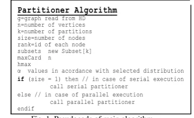
The main algorithm of the partitions consists of two main parts. The first one is executed if the number of nodes used in the cluster is equal to one, thus configuring a serial execution. The second main part of the algorithm is executed if the number of nodes to be used in the cluster is greater than one, thereby constituting a parallel execution. The main algorithm is shown in Fig. 1.
Partitioner Algorithm g=graph read from HD n=number of vertices k=number of partitions size=number of nodes rank=id of each node subsets new Subset[k] maxCard n
hmax
α values in acordance with selected distribution
if (size = 1) then// in case of serial execution call serial partitioner
else// in case of parallel execution call parallel partitioner endif
Fig. 1. Pseudocode of main algorithm.
The parallel algorithm is implemented as follows: two loops determine the number of times that the algorithm is executed. The external loop with h rounds will be executed hmax=log2k times, where k is the final number of partitions of the graph. For each iteration of this external loop, an internal loop runs 2h times. The internal loop initializes the number of threads specified for execution. Each thread then will run a number of iterations of partitioning determined by configuration and its related improvement routines to improve the cut-size. At the end of execution, each thread will have obtained its best cut in that round. This scheme is shown in Fig. 2.
Fig. 2. Node execution of threads and iterations.
The algorithm takes the smaller cut numbers between all threads, and stores the initial and final partitions and the border of the new created partition, since they will serve as input parameters for the next round, if the number of partitions of the graph (k) is greater than 2.
At the beginning, initial partition has all vertices of the graph and final partition is empty. At the end of the iteration, both partitions have half of the vertices of the initial partition, with a difference of at most one vertex. The total value of the cut-size of the graph is added to the value of this obtained smaller cut after the execution of the threads and their interactions. A new round h begins if k > 2. (See Fig. 3).
Fig. 3. Example of serial partition with 8 partitions.
On each node of the cluster, threads are also initialized depending on the number of processors and cores of the node, allowing further iterations in an attempt to obtain the lowest cut. On each processor in each node of the cluster, the algorithm behaves exactly as in the serial version.
In the parallel implementation, the parallel partitioner also runs the main external loop hmax = log2k times, where k is the final number of partitions of the graph. An important difference with respect to the serial solutions remains in the fact that the parallel partitioner distributes pairs of partitions according to specific distribution rules, while the serial partitioner works with all partitions without distinction.
The rules of distribution of partitions are as follow: in the first round of execution (h=0), every p (where p is the number of nodes in the cluster) nodes in the cluster receive the initial and final partitions equal to 0 (containing the vertices before partitioning) and 1 (empty before partitions), respectively. All nodes work in parallel trying to find the lowest cutting and its corresponding partitions. All nodes send their best cuts to the root node and the node with the lowest cut-size sends its initial (0) and final (1) partitions to the root node.
In the next round of execution (h=1), the nodes numbered (ranked) between 0 and (p/2-1) receive partitions 0 (containing one of the partitions obtained in the previous round) and 2 (empty before partitioning), while nodes with rank between (p/2) and (p -1) receive partition 1 (containing the other partition obtained in the previous round) and 3 (empty before partitioning).
Now, there are two halves of the cluster nodes working in parallel to calculate the smaller cut number between partitions 0 and 2 and between partitions 1 and 3. All nodes send to the root node their best cuttings. Finally, the root takes from all nodes the partitions 0, 1, 2 and 3 with the smallest calculated cut-size.
In the following rounds, the process is repeated such that in each round the number of nodes that perform the partitioning of each pair of partitions is halved while the number of partitions obtained in each round is duplicated.
VI. RESULTS
The algorithms proposed by [5] showed best results for graph bisection when compared to multilevel Metis and Chaco. According to the study proposed by [5], the Heuristic 3 seems to be the best solution considering overall results. Because they are multistart algorithms, the serial version had to run 10 times, with 100 iterations in each one, in order to obtain the best solution.
Likewise, the parallel version of Heuristic 3 was executed 10 times, with 100 iterations in each one, with the difference that the execution was carried out in a cluster with 16 nodes, each one running 16 threads simultaneously, resulting in total 16×16×100=25, 600 iterations. The smaller cut numbers are shown in the Table I.
TABLEI:BEST CUT-SIZE RESULTS FOR DIFFERENT HEURISTICS
Grafo Metis Chaco H3 Serial H3 Paralela
144 6871 6994 7248 7575
3elt 98 103 93 90
598a 2470 2484 2476 2463
add20 741 742 715 646
add32 19 11 11 11
airfoil1 85 82 77 74
bcsstk29 2923 3140 2885 2851
bcsstk33 12620 10172 10171 10171
Big 165 150 160 146
CCC5 28 29 16 16
crack 206 266 194 184
data 203 234 195 195
fe_rotor 2146 2230 2161 2107
fe_tooth 4198 4642 4113 3984
G124.04 65 65 63 63
G124.16 462 465 449 449
G250.08 860 845 828 828
G500.02 661 636 630 628
Grid32x32 32 34 32 32
memplus 6671 7549 6534 6524
nasa1824 757 824 739 739
nasa2146 882 870 870 870
stufe 19 20 16 16
U1000.20 222 286 222 222
U1000.40 812 895 737 737
U500.20 178 182 178 178
U500.40 412 412 412 412
vibrobox 11746 11196 10489 10343
whitaker 128 133 128 127
wing_nodal 1848 1850 1746 1727
The parallel solution for Heuristic 3 showed no improvement in the cut of the graph 144. Changes in the configuration of Heuristic 2 can result in a better cut. With only 10 runs of 10 iterations each, running in the same configuration of 16 nodes and 16 threads per node in the cluster, the cut of the graph has been improved, reaching the value of 6856.
Compared with the serial algorithms proposed, the total execution time of the parallel algorithm in the cluster was higher. But, in essence, we are comparing only 100 iterations of the serial solution against 25,600 iterations of the parallel algorithm. In the analysis of speedup, when comparing the number of iteration of boot solutions, the parallel solution presents a significant gain of time and improve the quality of the cut.
In addition to the improvements made in the cuts of bisections, the parallel algorithm brought significant gains in speedup. For an increasing number of iterations, the purely serial implementation would become unworkable in practice, however, the parallel algorithms using both a number of nodes in a cluster and also a number of threads in each processing node, made the execution times dropped considerably.
iterations that were considered for performance evaluation. For each configuration named by the attribute "name", 6400 iterations are performed. Note that the configuration 01n01t simulates serial execution and the others its parallel execution in terms of number of processing nodes and threads used.
TABLEII:TEST SCENARIOS
Name Number of nodes Threads Iterations Total
01n01t 1 1 6.400 6.400
01n16t 1 16 400 6.400
02n16t 2 16 200 6.400
04n16t 4 16 100 6.400
08n16t 8 16 50 6.400
Table III shows the execution times, in seconds, for the different configurations performed for each graph analyzed.
TABLEIII:EXECUTION TIME FOR DIFFERENT SCENARIOS
Grafo 01n01t 01n16t 02n16t 04n16t 08n16t
144 9.987,645 2.267,888 1.825,586 902,987 446,436
3elt 21,511 5,924 3,569 3,318 1,859
598a 4.884,235 1.222,244 868,995 428,393 218,654
add20 12,979 3,608 2,506 1,796 1,431
add32 12,979 3,608 2,506 1,796 1,431
airfoil1 19,142 4,206 3,226 2,367 2,419
bcsstk29 866,845 158,465 118,764 60,845 30,567
bcsstk33 1.367,146 254,094 187,402 96,084 49,175
Big 84,805 18,077 13,100 7,111 3,701
CCC5 0,685 1,038 0,693 0,567 0,397
crack 48,378 9,636 7,439 4,091 2,509
data 20,819 5,546 4,352 2,161 1,981
fe_rotor 3.004,040 662,326 466,571 246,643 136,502
fe_tooth 1.976,274 424,307 327,463 160,237 86,213
G124.04 1,756 2,376 1,505 0,821 0,500
G124.16 8,213 3,839 3,390 2,601 1,688
G250.08 18,794 4,082 2,923 2,560 2,776
G500.02 18,950 5,430 2,837 2,995 2,488
Grid32x32 2,573 1,950 1,461 0,923 0,673
memplus 461,985 55,835 49,664 25,236 12,937
nasa1824 44,388 6,702 6,515 3,753 2,385
nasa2146 62,561 10,690 8,743 4,930 2,897
stufe 4,101 2,403 2,451 1,400 0,904
U1000.20 9,323 3,625 1,787 2,190 1,317
U1000.40 23,575 5,438 3,797 2,721 1,566
U500.20 17,791 6,243 3,048 2,861 1,850
U500.40 46,273 7,482 6,835 3,998 2,301
vibrobox 1.449,632 218,383 205,925 105,042 51,749
whitaker 37,238 8,581 6,183 3,491 2,306
wing_nodal 270,458 40,898 36,566 19,026 9,860
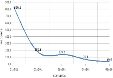
Fig. 4 shows the average execution time of all graphs for each configuration. The curve shows a natural decrease of the execution time with the increasing number of execution nodes and threads.
As a result, the parallelization achieves a very good rate of speedup, as can be showed in Fig. 5. For example, in the simplest scenario, running the heuristic using 1 node and 16 threads (01n16t) the speed is multiplied by 4. As we added more nodes, the speed of execution increases until it reaches the value of 15, 6 times the serial speed (08n16t).
Fig. 4. Average execution time for different scenarios showed in Table II.
Fig. 5. Average speedup for different scenarios from Table II.
Note that Fig. 5 shows the average speedup for running the parallel solution for all graphs. To calculate the speedup for each graph you should use equation (1). For example, the speedup of graph 144 running scenario 08n16t is:
S8= T01n01t / T08n16t = 9.987,645 / 446,436 = 22, 37
VII. GPPAPPLIED TO MULTIPHASE FLOW SIMULATION
We applied this solution to generate partitions of a big graph which is the result of the discretizations process of the simulation domain of a problem of multiphase flows in porous media to oil recovery. This previous step is necessary in order to generate groups of data to be processed in a paralleling simulation. The results in terms of processing time and cut-size have shown it is a very efficient solution when compared with serial algorithms, as shown in Table I.
VIII. CONCLUSION
Optimal solutions to graph partitioning with high numbers of vertices become computationally infeasible in practice. Several heuristics and metaheuristics have been proposed to overcome this difficulty.
Additionally, parallel algorithmic techniques for execution on parallel machines can be used to decrease computational time.
The present work proposes an efficient parallel solution to the GPP problem based on the implementation of existing heuristics in a computational cluster with identical processing nodes based on Intel QuadCore processors and supported by MPIJava programming platform. The proposed solution improves the general performance of the heuristics presented in [5] in two aspects: 1) improvement of the execution time, with a considerable speedup related to the serial solution and, 2) improvement of the quality of the created partitions, by introducing some random features into the original heuristics. After parallelization of the heuristics proposed by [5], the performance of the parallel solution of Heuristic 3 showed improvement in 50% of the cut-size of the graphs when compared to serial algorithms. In the remaining 50%, the cuts were at least equal, never worse than in the other serial algorithms.
greedy, was more appropriated. The main focus of this work was to improve the cut-size of the partitioning graph problem. However, time savings were also obtained when comparing the execution of the same number of iterations of the algorithm on an isolated node of the cluster (monothread and serial execution) with the implementation of 16 nodes, each running 16 threads in parallel.
REFERENCES
[1] P. O. Fjallstrom, “Algorithms for graph partitioning: a survey,” Linkoping Electronic Articles in Computer and Information Science, vol. 3, no. 10, 1998.
[2] T. N. Bui and B. R. Moon, “Genetic algorithm and graph partiotining,” IEEE Transactions and Computers, no. 45, pp. 841-855, 1996. [3] R. S. Bonatto and A. R. S. Amaral, “Algoritmo heurístico para partição
de grafos com aplicação em processamento paralelo,” presented at XLII Congresso da Sociedade Brasileira de Pesquisa Operacional, RJ, 2010.
[4] S. E. Schaeffer, “Graph clustering,” Computer Science Review, no 1, pp. 27-64, 2007.
[5] R. S. Bonatto, “Algoritmos heurísticos para partição de grafos com aplicação em processamento paralelo,” M.S. thesis, Dept. Computing, ES Federal Univ., Vitória, Brazil, 2010.
[6] K. Schloegel, G. Karypis, and V. Kumar, Graph Partitioning for High Performance Scientific Simulations, Sourcebook of Parallel Computing, San Francisco, CA: Morgan Kaufmann Publishers Inc., 2003.
[7] C. Ou and S. Ranka, “SPRINT: scalable partitioning, refinement, and incremental partitioning techniques,” unpublished.
[8] G. Karypis and V. Kumar, “A fast and high quality multilevel scheme for partitioning irregular graphs,” Siam J. Sci Comput., vol. 20, no. 1, pp. 359-392, 1998.
[9] G. Karypis and V. Kumar, “Multilevel k-way partitioning scheme for irregular graphs,” Journal of Parallel and Distributed Computing, no. 48, pp. 96-129, 1998.
[10] S. Guattery and G. L. Miller, “On the performance of spectral graph partitioning methods,” in Proc. 2th Ann. ACM/SIAM Symposium on Discrete Algorithms, California, 1995, pp. 233-242.
[11] H. Qiu and E. R. Hancock, “Graph matching and clustering using spectral partitions,” Journal of Pattern Recognition, no. 39, pp. 22-24, 2006.
[12] U. Benlic and J. K. Hao, “Hybrid metaheuristics for the graph partitioning problem,” unpublished.
[13] C. Fiduccia and R. Mattheyeses, “A linear-time heuristic for improving network partitions,” in Proc. 19th IEEE Design Automation Conference, Las Vegas, USA, 1982, pp. 175-181.
[14] B. W. Kernighan and S. Lin, “An efficient heuristic procedure for partitioning graphs,” Bell System Technical Journal, vol. 49, no. 1, pp. 291-307, 1970.
[15] D. S. Johnson, C. R. Aragon, L. A. McGeoch, and C. Schevon, “Optimizationby simulated annealing: an experimental evaluation; part I, graph partitioning,” Journal of Operations Research, no. 37, pp. 865-892, 1989.
[16] E. Rolland, H. Pirkul, and F. Glover, “Tabu search for graph partiotining,” Annals of Operations Research, no. 63, pp. 209-232, 1996.
Roney Pignaton da Silva was born on August 4th, 1972 in São Mateus, ES. Graduated with a BS from Federal University of ES, Brazil in 1997, a MS from the Federal University of ES, Brazil in 1999, and a PhD from Polytechnic University of Madrid, Spain in 2004.