© 2017 IJSRSET | Volume 3 | Issue 2 | Print ISSN: 2395-1990 | Online ISSN : 2394-4099 Themed Section: Engineering and Technology
Advanced Algorithm for Reduction of Real Power Loss
Dr. K. Lenin
Researcher, JNTU, Hyderabad, Andhra Pradesh, India
ABSTRACT
This paper projects Enriched Monkey Algorithm (EMA) for solving the Reactive Power problem. The crucial feature in this problem is to reduce the real power loss and to keep voltage profiles within limits. This algorithm is stimulated from the mountain climbing procedures of monkeys where the monkeys look for the highest mountain by climbing up from their present position. The simulation results expose amended performance of the EMA in solving an optimal reactive power problem. In order to evaluate up the performance of the proposed algorithm, it has been tested on Standard IEEE 57,118 & practical 191 bus systems. It has been compared to other reported standard algorithms. Simulation results show that EMA is better than other algorithms in plummeting real power loss and voltage profiles also within the limits.
Keywords: EnrichedMonkey Algorithm, Optimization, Optimal Reactive Power, Transmission Loss.
I.
INTRODUCTION
Optimal reactive power problem plays most significant role in the stability of power system operation and control. In this paper the key aspect is to reduce the real power loss and to keep the voltage variables within the limits. Formerly many mathematical methods like gradient method, Newton method, linear programming [1-7] has been employed to solve the optimal reactive power dispatch problem and those approaches have many complications in handling inequality constraints. Voltage stability and voltage collapse play an imperious role in power system planning and operation [8]. Newly Evolutionary algorithms like genetic algorithm have been already employed to solve the reactive power flow problem [9,10].In [11-20] Genetic algorithm, Hybrid differential evolution algorithm, Biogeography Based algorithm, fuzzy based methodology, improved evolutionary programming has been used to solve optimal reactive power flow problem and all the algorithm efficaciously handled the reactive power problem.In this paper the Enriched Monkey Algorithm (EMA) [21], is used to solve the optimal reactive power problem. The performance of EMA has been evaluated in standard IEEE 57,118& 191 practical test systems and the simulation results shows that our proposed
method outperforms all approaches investigated in this paper.
II.
OBJECTIVE FUNCTION
A. Active power loss
The objective of the reactive power dispatch problem is to minimize the active power loss and can be written in equations as follows:
F = 𝑃𝐿= ∑k∈Nbr gk(Vi2+ V
j2− 2ViVjcosθij) (1)
Where F- objective function, PL – power loss, gk -
conductance of branch,Vi and Vj are voltages at buses i,j,
Nbr- total number of transmission lines in power systems.
B. Voltage profile improvement
To minimize the voltage deviation in PQ buses, the objective function (F) can be written as:
Where VD - voltage deviation, ωv- is a weighting factor of voltage deviation.
And the Voltage deviation given by:
VD = ∑Npqi=1|Vi− 1| (3)
Where Npq- number of load buses
C. Equality Constraint
The equality constraint of the problem is indicated by the power balance equation as follows:
PG= PD+ PL (4)
Where PG- total power generation, PD - total power
demand.
D. Inequality Constraints
The inequality constraint implies the limits on components in the power system in addition to the limits created to make sure system security. Upper and lower bounds on the active power of slack bus (Pg), and
reactive power of generators (Qg) are written as follows:
Pgslackmin ≤ P
gslack ≤ Pgslackmax (5)
Qmingi ≤ Qgi≤ Qgimax , i ∈ Ng (6)
Upper and lower bounds on the bus voltage magnitudes (Vi) is given by:
Vimin≤ Vi≤ Vimax , i ∈ N (7)
Upper and lower bounds on the transformers tap ratios (Ti) is given by:
Timin≤ Ti≤ Timax , i ∈ NT (8)
Upper and lower bounds on the compensators (Qc) is
given by:
Qcmin≤ Q
c≤ QCmax , i ∈ NC (9) Where N is the total number of buses, Ng is the total
number of generators, NT is the total number of
Transformers, Nc is the total number of shunt reactive
compensators.
III.
Monkey Algorithm
The Monkey Algorithm (MA) is stimulated from the mountain climbing procedure of monkeys, where the monkeys look for the highest mountain by climbing up from their positions. When each monkey gets to the top of the mountain, it looks about to find out whether there are higher mountains around or not. If yes, it will jump toward the mountain from the current position and then replicate the climbing until it reaches the top of the higher mountain. The MA is based on three main process namely as climb process, watch-jump process and somersault process. In following the monkey algorithm, the proposed EMA for optimal reactive power dispatch has been explained.
A. Standard Monkey Algorithm
Generally the monkey algorithm [21] works as follows, Step 1: Describe the population size of monkeys (M), the climb number (Nc), the objective function and the
decision variables. Give the Input about system parameters and the boundaries of the decision variables. The optimization problem can be defined as:
Minimization f(x)
Subject to
𝐿 ≤ ≤ (10)
Where ( =1,2,..,n), 𝐿 and lower and upper bounds of decision variables.
Step2 : Initialize a possible position for each monkey, where the position of ith monkey is denoted as a vector with n dimension:
= ( 1, 2, , ) , = 1,2, , (11)
Step 3. Climb procedure is a step by step procedure to change the monkeys' positions from the initial positions to new ones that makes an improvement in the objective function
The climb process can be explained in three stages
Stage 1 - Generate a vector randomly
Where
= {+ (+ ) = − 𝑃(− ) = (13)
a – step length of climb process.
Stage 2 -To calculate the simulated gradient of the objective function at point
= ( ) ( )
2 , = 1,2, , (14)
= ( 1( ), 2( ), , ( )) (15)
Stage 3 – Describe the parameter = ( 1, 2, ) and it can be calculated as follows,
= + ( ( )) , = 1,2, , (16)
If = ( 1, 2, ) is feasible then is replaced by , otherwise remains the same .
Stage 1to 3 are repeated until there is no considerable changes on the values of objective function or the climb number Ncis reached.
Step 4. After the climb process, each monkey arrives at its own mountaintop, therefore; each monkey will look around to find a higher mountain. If a higher mountain is found, the monkey will jump there (jump process). For this a parameter b is defined as eyesight of the monkey which is the maximal distance that the monkey can watch.
The jump is based on two stages
Stage 1- A real number y is generated randomly in the range of :
∈ ( − , + ) , = 1,2, , (17)
Stage 2-If y is feasible and f(y) is better than f(x) for ith monkey (f(y) > f(x)), the position is updated; otherwise, Stage 1 is repeated.
Step 5. The climb process is repeated by considering y
as initial position.
Step 6. Somersault procedure: In this step, the monkeys find out new penetrating domain. Taking the centre of all the monkeys‟ positions as a pivot, each monkey will somersault to a new position forward or backward in the direction of pointing at the pivot. Based on the new position, the monkeys will keep on climbing. The somersault procedure is as follows:
Stage 1-First a somersault interval [c, d] is defined which the maximum distance that monkeys can somersault is. A real number is generated randomly within the somersault interval.
= + (𝑃 − ) (18)
𝑃 = 1∑ =1 , = 1,2, , (19)
Where P is somersault pivot.
Stage 3- If = ( 1, 2, ) is feasible then is replaced by , otherwise remains the same.
Step 7. Repeat steps 3-6 until the stopping criterion (maximum number of iteration) is met.
IV.
Enriched Monkey Algorithm (EMA)
To have a high performance search, an essential key is having an appropriate transaction between exploration and exploitation. Monkey Algorithm may fall into a local optimum early in a run on some optimization problems. In other words, the algorithm approaches the neighbourhood of the global optimum but for some reasons it fails to converge to the global optimum. The stagnation could be due to the following reason:
Monkeys don‟t share information and learning from each other, so this easily makes the algorithm to trap in the local optimum solution .Also the improvement in the position is in the range of − , + and it has been done randomly. So the time process will be higher one to find better solution .In this EMA rather than going randomly by each monkey based on local information, the information has been transferred and a common decision has been made by obtaining the information from other monkeys as below
= + ( − ) (20)
Where
= 1,2, ,
= 1,2, ,
= 1,2, , ,
- Random number in the range of [-1,1], −are chosen randomly in the range of *1,2, , +.
If the new position is better than previous position then the monkey will jump otherwise the position remains unchanged. But the monkey will try to improve the position by using the step.
= (22)
EMA for solving reactive power dispatch problem,
Initiate
Scrutinize the data and identify constraint Reset the parameter
Modernize iteration count up Climb technique
Somersault technique
Appraise the monkey position using the new-fangled search operator
If it meets stopping criterion process stop or go again to climb procedure.
End
V.
Simulation Results
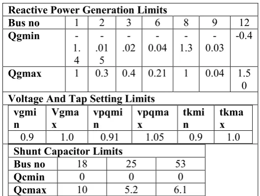
ProposedEnriched Monkey Algorithm (EMA) is tested in standard IEEE-57 bus power system. The reactive power compensation buses are 18, 25 and 53. Bus 2, 3, 6, 8, 9 and 12 are PV buses and bus 1 is selected as slack-bus. The system variable limits are given in Table 1.
The preliminary conditions for the IEEE-57 bus power system are given as follows:
Pload = 12.328 p.u. Qload = 3.124 p.u.
The total initial generations and power losses are obtained as follows:
∑ 𝑃 = 12.6716 p.u. ∑ = 3.3412 p.u. Ploss = 0.26427 p.u. Qloss = -1.2047 p.u.
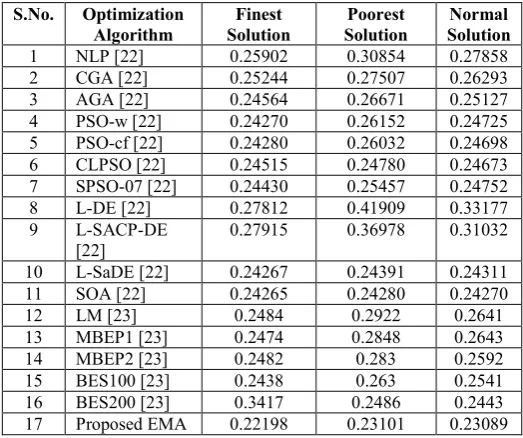
Table 2 shows the various system control variables i.e. generator bus voltages, shunt capacitances and transformer tap settings obtained after EMA based optimization which are within the acceptable limits. In Table 3, shows the comparison of optimum results obtained from proposed EMA with other optimization techniques. These results indicate the robustness of proposed EMA approach for providing better optimal solution in case of IEEE-57 bus system.
TABLE 1.VARIABLE LIMITS
Reactive Power Generation Limits
Bus no 1 2 3 6 8 9 12
Qgmin
-1. 4
-.01
5 -.02
-0.04
-1.3
-0.03
-0.4
Qgmax 1 0.3 0.4 0.21 1 0.04 1.5
0
Voltage And Tap Setting Limits vgmi
n Vgmax vpqmin vpqmax tkmin tkmax
0.9 1.0 0.91 1.05 0.9 1.0
Shunt Capacitor Limits
Bus no 18 25 53
Qcmin 0 0 0
Qcmax 10 5.2 6.1
TABLE 2.CONTROL VARIABLES OBTAINED AFTER OPTIMIZATION
Control
Variables
EMA
V1
1.1
V2
1.051
V3
1.057
V6
1.012
V8
1.040
V9
1.021
V12
1.020
Qc18
0.0698
Qc25
0.202
Qc53
0.0489
T4-18
1.010
T21-20
1.059
T24-25
0.899
T24-26
0.892
T7-29
1.079
T34-32
0.893
T11-41
1.014
T15-45
1.040
T14-46
0.911
T10-51
1.022
T13-49
1.061
T11-43
0.910
T40-56
0.901
T39-57
0.951
TABLE 3.COMPARISON RESULTS
S.No. Optimization Algorithm
Finest Solution
Poorest Solution
Normal Solution
1 NLP [22] 0.25902 0.30854 0.27858 2 CGA [22] 0.25244 0.27507 0.26293 3 AGA [22] 0.24564 0.26671 0.25127 4 PSO-w [22] 0.24270 0.26152 0.24725 5 PSO-cf [22] 0.24280 0.26032 0.24698 6 CLPSO [22] 0.24515 0.24780 0.24673 7 SPSO-07 [22] 0.24430 0.25457 0.24752 8 L-DE [22] 0.27812 0.41909 0.33177 9 L-SACP-DE
[22]
0.27915 0.36978 0.31032 10 L-SaDE [22] 0.24267 0.24391 0.24311 11 SOA [22] 0.24265 0.24280 0.24270 12 LM [23] 0.2484 0.2922 0.2641 13 MBEP1 [23] 0.2474 0.2848 0.2643 14 MBEP2 [23] 0.2482 0.283 0.2592 15 BES100 [23] 0.2438 0.263 0.2541 16 BES200 [23] 0.3417 0.2486 0.2443 17 Proposed EMA 0.22198 0.23101 0.23089
Then Enriched Monkey Algorithm (EMA) has been tested in standard IEEE 118-bus test system [24] .The system has 54 generator buses, 64 load buses, 186 branches and 9 of them are with the tap setting transformers. The limits of voltage on generator buses are 0.95 -1.1 per-unit., and on load buses are 0.95 -1.05 per-unit. The limit of transformer rate is 0.9 -1.1, with the changes step of 0.025. The limitations of reactive power source are listed in Table 4, with the change in step of 0.01.
TABLE 4.LIMITATION OF REACTIVE POWER SOURCES
BUS 5 34 37 44 45 46 48
QCMAX 0 14 0 10 10 10 15
QCMIN -40 0 -25 0 0 0 0
BUS 74 79 82 83 105 107 110
QCMAX 12 20 20 10 20 6 6
QCMIN 0 0 0 0 0 0 0
The statistical comparison results of 50 trial runs have been list in Table 5 and the results clearly show the better performance of proposed EMA algorithm.
TABLE 5.COMPARISON RESULTS
Active power
loss (p.u) BBO [25] ILSBBO/ strategy1 [25]
ILSBBO/ strategy1
[25]
Proposed EMA
Min 128.77 126.98 124.78 117.61
Max 132.64 137.34 132.39 121.59
Average 130.21 130.37 129.22 118.99
Finally Enriched Monkey Algorithm (EMA) has been tested in practical 191 test system and the following results has been obtained
In Practical 191 test bus system – Number of Generators = 20, Number of lines = 200, Number of buses = 191 Number of transmission lines = 55.
Table 6 shows the optimal control values of practical 191 test system obtained by EMA method. And table 7 shows the results about the value of the real power loss by obtained byEnriched Monkey Algorithm (EMA).
TABLE 6.OPTIMAL CONTROL VALUES OF PRACTICAL 191
UTILITY (INDIAN) SYSTEM BY EMA METHOD
VG1 1.11 VG 11 0.90
VG 2 0.81 VG 12 1.00
VG 3 1.02 VG 13 1.01
VG 4 1.01 VG 14 0.91
VG 5 1.10 VG 15 1.01
VG 6 1.14 VG 16 1.03
VG 7 1.10 VG 17 0.90
VG 8 1.01 VG 18 1.00
VG 9 1.10 VG 19 1.11
VG 10 1.02 VG 20 1.10
T1 1.00 T21 0.90 T41 0.90
T2 1.04 T22 0.91 T42 0.90
T3 1.01 T23 0.92 T43 0.91
T4 1.10 T24 0.90 T44 0.91
T5 1.00 T25 0.90 T45 0.91
T6 1.01 T26 1.00 T46 0.90
T7 1.00 T27 0.91 T47 0.92
T8 1.02 T28 0.90 T48 1.00
T10 1.00 T30 0.90 T50 0.91
T11 0.90 T31 0.91 T51 0.90
T12 1.01 T32 0.91 T52 0.90
T13 1.02 T33 1.03 T53 1.00
T14 1.01 T34 0.92 T54 0.90
T15 1.01 T35 0.90 T55 0.90
T19 1.02 T39 0.94
T20 1.03 T40 0.90
TABLE 7.OPTIMUM REAL POWER LOSS VALUES OBTAINED FOR PRACTICAL 191 UTILITY (INDIAN)
SYSTEM BY EMA METHOD.
Real power Loss (MW)
EMA
Min 146.592
Max 149.712
Average 147.989
VI.
CONCLUSION
In this Enriched Monkey Algorithm (EMA) approach efficiently solved optimal reactive power problem. The performance of the proposed Enriched Monkey Algorithm (EMA) has been demonstrated by testing it in IEEE 57,118 & practical 191 test bus systems. Simulation results shows that Real power loss has been considerably reduced and voltage profiles are within the specified limits.
VII.
REFERENCES
[1] O. Alsac,and B. Scott, “Optimal load flow with steady state security”,IEEE Transaction. PAS -1973, pp. 745-751.
[2] Lee K Y ,Paru Y M , Oritz J L –A united approach to optimal real and reactive power dispatch , IEEE Transactions on power Apparatus and systems 1985: PAS-104 : 1147-1153
[3] A.Monticelli , M .V.F Pereira ,and S. Granville , “Security constrained optimal power flow with post contingency corrective rescheduling” , IEEE Transactions on Power Systems :PWRS-2, No. 1, pp.175-182.,1987.
[4] DeebN ,Shahidehpur S.M ,Linear reactive power optimization in a large power network using the decomposition approach. IEEE Transactions on power system 1990: 5(2) : 428-435
[5] E. Hobson ,‟Network consrained reactive power control using linear programming, „ IEEE Transactions on power systems PAS -99 (4) ,pp 868=877, 1980
[6] K.Y Lee ,Y.M Park , and J.L Oritz, “Fuel –cost optimization for both real and reactive power dispatches” , IEE Proc; 131C,(3), pp.85-93. [7] M.K. Mangoli, and K.Y. Lee, “Optimal real and
reactive power control using linear programming” ,Electr.PowerSyst.Res, Vol.26, pp.1-10,1993. [8] C.A. Canizares , A.C.Z.de Souza and V.H.
Quintana , “ Comparison of performance indices for detection of proximity to voltage collapse ,‟‟ vol. 11. no.3 , pp.1441-1450, Aug 1996 .
[9] Eleftherios I. Amoiralis, Pavlos S. Georgilakis, Marina A. Tsili, Antonios G. Kladas,(2010), “Ant Colony Optimisation solution to distribution transformer planning problem”, Internationl Journal of Advanced Intelligence Paradigms , Vol.2, No.4 ,pp.316 – 335.
[10] D. Devaraj, and B. Yeganarayana, “Genetic algorithm based optimal power flow for security enhancement”, IEE proc-Generation.Transmission and. Distribution; 152, 6 November 2005.
[11] Berizzi, C. Bovo, M. Merlo, and M. Delfanti, “A ga approach to compare orpf objective functions including secondary voltage regulation,” Electric Power Systems Research, vol. 84, no. 1, pp. 187 – 194, 2012.
[12] C.-F. Yang, G. G. Lai, C.-H. Lee, C.-T. Su, and G. W. Chang, “Optimal setting of reactive compensation devices with an improved voltage stability index for voltage stability enhancement,” International Journal of Electrical Power and Energy Systems, vol. 37, no. 1, pp. 50 – 57, 2012. [13] P. Roy, S. Ghoshal, and S. Thakur, “Optimal var
[14] Venkatesh, G. Sadasivam, and M. Khan, “A new optimal reactive power scheduling method for loss minimization and voltage stability margin maximization using successive multi-objective fuzzy lp technique,” IEEE Transactions on Power Systems, vol. 15, no. 2, pp. 844 – 851, may 2000. [15] W. Yan, S. Lu, and D. Yu, “A novel optimal
reactive power dispatch method based on an improved hybrid evolutionary programming technique,” IEEE Transactions on Power Systems, vol. 19, no. 2, pp. 913 – 918, may 2004. [16] W. Yan, F. Liu, C. Chung, and K. Wong, “A
hybrid genetic algorithminterior point method for optimal reactive power flow,” IEEE Transactions on Power Systems, vol. 21, no. 3, pp. 1163 –1169, aug. 2006.
[17] J. Yu, W. Yan, W. Li, C. Chung, and K. Wong, “An unfixed piecewiseoptimal reactive power-flow model and its algorithm for ac-dc systems,” IEEE Transactions on Power Systems, vol. 23, no. 1, pp. 170 –176, feb. 2008.
[18] F. Capitanescu, “Assessing reactive power reserves with respect to operating constraints and voltage stability,” IEEE Transactions on Power Systems, vol. 26, no. 4, pp. 2224–2234, nov. 2011.
[19] Z. Hu, X. Wang, and G. Taylor, “Stochastic optimal reactive power dispatch: Formulation and solution method,” International Journal of Electrical Power and Energy Systems, vol. 32, no. 6, pp. 615 – 621, 2010.
[20] Kargarian, M. Raoofat, and M. Mohammadi, “Probabilistic reactive power procurement in hybrid electricity markets with uncertain loads,” Electric Power Systems Research, vol. 82, no. 1, pp. 68 – 80, 2012.
[21] R. Zhao, W. Tang, “Monkey Algorithm for Global Numerical Optimization”, Journal of Uncertain Systems, Vol. 2, Issue 3, pp. 165-176, 2008.
[22] Chaohua Dai, Weirong Chen, Yunfang Zhu, and Xuexia Zhang, “Seeker optimization algorithm for optimal reactive power dispatch,” IEEE Trans. Power Systems, Vol. 24, No. 3, August 2009, pp. 1218-1231.
[23] J. R. Gomes and 0. R. Saavedra, “Optimal reactive power dispatch using evolutionary computation: Extended algorithms,” IEE Proc.-Gener. Transm. Distrib.. Vol. 146, No. 6. Nov. 1999.
[24] IEEE, “The IEEE 30-bus test system and the
IEEE 118-test system”, (1993),
http://www.ee.washington.edu/trsearch/pstca/. [25] Jiangtao Cao, Fuli Wang and Ping Li, “An