Abstract—These Images of the inside of the human body can be obtained using tomographic acquisition and processing techniques. In particular, these techniques are commonly used to obtain X_ray images of the human body. The reconstructed images are obtained given a set of their projections, acquired using reconstruction techniques. A general overview of analytical and iterative methods of reconstruction in computed tomography (CT) is presented in this paper, with a special focus on Bayesian algorithms. The simulated results are compared using quality measurements for various test cases and conclusion is achieved. Through these simulated results, we have demonstrated that the Bayesian approach provides the best image quality and the small values of the quality measurements.
Index Terms—Computed tomography, bayesian approach, reconstruction techniques.
I. INTRODUCTION
During the last decade, there has been an avalanche of publications on different aspects of computed tomography [1]-[3]. The word tomography means reconstruction from slices. It is an imaging technique which uses the absorption of X-rays by a number of organs in the body. In tomography, images coming from the computed tomography scan are combined to create a visualization of the scanned body. To create this image we use reconstruction techniques. The conventional algorithms of image reconstruction for CT are backprojection (BP) and Filtered Back Projection (FBP) reconstruction techniques which are analytical reconstruction methods [4]. Many efforts are also being made to make iterative methods popular again due to their unique advantages, such as their performances with incomplete noisy data. One of the most important iterative reconstruction techniques in CT is the conjugate gradient (CG) algorithm [2]. It is considered as an optimization method. More recently, stochastic methods, which are based on the Bayesian framework, have been successfully used in CT [3].
This article presents the basics of the more widely used algorithms: backprojection (BP), filtered backprojection
Manuscript received April 15, 2012; revised June 5, 2012. This work was supported in part by the Ministry of Higher Education and Scientific Research, ALGERIA, under Grant Cerist 15/TIC/2011.
Z. Messali is with the Department of Electronics, Bordj Bou Arréridj, 34265 ALGERIA (e-mail: [email protected]).
N. Chetih and A. Serir are with the Department of Electronics, Algiers, 16000, ALGERIA (e-mail: [email protected], [email protected]).
A. Boudjelal is with the Department of Electronics, M’Sila, 28000, ALGERIA (e-mail: [email protected])
(FBP), Gradient algorithms and a special focus on a Bayesian maximum a posteriori (MAP) approach. Therefore, this paper is aimed to establish a comparative study of analytical and iterative reconstruction techniques in order to reduce the number of iterations and enhance the image quality. We concentrate on the Bayesian approach. Two Phantoms are used to test the results of the research: the Shepp-Logan head model phantom and the standard medical image of abdomen (see Fig. 1). We present the reconstruction techniques in section 2 and 3 respectively. We focus on developing a Bayesian MAP (maximum a posteriori) approach in section 4, in which the reconstruction is computed by maximizing an associated objective function via an iterative algorithm. Following this, in section 5, we explain how to evaluate the quality of the reconstruction. Section 6 provides some test results and comparisons. Finally, in the last section our conclusions can be read.
II. ANALYTICAL RECONSTRUCTION METHODS
The projections (or line integral), are defined as p t f x yds
t
∫
= ( ,) ( , ) )
(
θ
θ (1) The function pθ(t) is known as the Radon transform of the function f(x,y), where f(x,y) represents the 2D image to be reconstructed, and (θ,t) the parameters of each line integral. (θ,t) is also known as a sinogram of the image. It is well known that, from knowledge of the sinogram pθ(t), one can readily reconstruct the image f(x,y) by use of computationally efficient and numerically stable algorithms such as the backprojection (BP) and filtered backprojection (FBP) algorithm. These two algorithms will be described in the following.
A. Backprojection (BP)
In order to recover the image from its Radon transform, we simply apply back projection. The backprojection operation is defined as:
= =
∫
π θ θ0 ( )
) , ( ˆ ) ,
(x y f x y p t d
b (2) Backprojection represents the accumulation of the ray-sums of all the rays that pass through any point. Applying backprojection to projection data is called the summation algorithm. However, applying backprojection to the function
A Comparative Study of Analytical, Iterative and Bayesian
Reconstruction Algorithms in Computed Tomography
(CT)
) (t
pθ does not yield f(x,y) but a blurred f(x,y) as it will be shown in our simulation results.
B. Filtered Backprojection (FBP )
The Filtered Backprojection approach is a direct method and capitalizes on the Fourier Slice Theorem [4] and the Radon transform. The Fourier Slice Theorem relates the Fourier transform of a projection to the Fourier transform of the object along a single radial. FBP is mathematically expressed as:
θ
π π
θ v v e dv d
p y
x
f j vt
∫ ∫
⎟ ⎠ ⎞ ⎜ ⎝ ⎛ ⋅ ⋅ = +∞ ∞ − 0 2 | | ) ( ) ,( (3)
where pθ(v) is 1D Fourier Transform of pθ(t), and |v| is the ramp filter.
III. ITERATIVE RECONSTRUCTION TECHNIQUES
A. Gradient Algorithm
In iterative methods, one wants to solve p=Af where p
is the vector of values in the sinogram, A is a given matrix, and f is the unknown vector of pixel values in the image to be reconstructed.
One of the iterative reconstruction techniques is the Gradient algorithm. Mathematically, the Gradient algorithm or steepest-descent algorithm iteratively searches for f
using the equation:
) ( ) ( ) ( ) 1
(k f k k pk
f + = +α (4) This means that the new estimate f(k+1) is equal to previous estimate f(k) plus a vector p(k) indicating the new direction (chosen to be opposite to the local gradient, and therefore directed toward the steepest descent), weighted by a coefficient α(k) representing the step length. The criterion of this algorithm is the progressive minimization of the difference between the measured projections and estimated ones. That is, the error is defined as:
p−Af 2 (5)
IV. BAYESIAN APPROACH
We consider the linear model with additive white Gaussian noise, i.e.,
p=Af +n (6) where p,f and n are vectors of random variables. In Bayesian inversion theory, the complete solution for an inverse problem is represented by the posterior distribution, given by Bayes’ formula
) / ( ) ( ) ( ) / ( ) ( ) /
( p f p p f
p p f p p f p p f
p = α (7)
where p(p/f) is the likelihood density, p(f) is the prior density and p(p) is normalization constant. We select the maximum a posteriori (MAP) estimate which is obtained from ) / ( max arg
ˆ p f p
f = f (8) It means that for the given prior density p(f) and the measurement datap, we determine the unknown values f
which are in the best agreement with the model (6). Assuming zero mean, isotropique Gaussian noise with variance 2
n
σ , the likelihood function is
⎟ ⎟ ⎠ ⎞ ⎜ ⎜ ⎝ ⎛ − − 2 2 2 exp ) / ( n Af p f p p σ
α (9)
The next question is how to choose the prior density function p(f). For simplicity, we select the Gaussian white noise prior with the positivity constraint, i.e.,
) ( 2 exp ) ( 2 2 f u f p p n ⎟ ⎟ ⎠ ⎞ ⎜ ⎜ ⎝ ⎛ − σ
α (10)
where the step function u(f) equals to one when all the elements in f are positive; otherwise it is zero. The computation of MAP implies minimizing
{
2 2}
min arg
ˆ p Af f
f = f − (11) +λ where the regularization parameter 2/ 2
f
n σ
σ
λ = . The higher the noise level, the larger the regularization parameterλ. At each iterationk, a current estimate of the image is available. The measured projections are then compared with simulated projections of the current estimate, and the error between these simulated and measured projections is used to modify the current estimate to produce an updated (and hopefully more accurate) estimate, which becomes iteration k+1. This process is then repeated many times.
V. PERFORMANCE EVALUATION
2 2 ˆ
f f f
df = − (12)
where f is the gray level value of the test image and fˆ is
the gray level value of the reconstructed image. The second criterion is the relative norm error of the simulated projections and defined a
2 2 ˆ
p p p
dp= − (13)
where p is the measured projection and pˆ is the simulated projection. Smaller errors dp and df means that the resulting reconstructed image is closer to the test image. Another criterion is the number of iterations. Smaller iteration is preferable. Projections (parallel beam type) for the image reconstruction are calculated analytically by defining the first test image: Shepp logan phantom head model (Simulated) image as it is shown in Fig. 1 (a). Fig. 1 (b) shows the second test image which is the standard medical image of abdomen. Projections are calculated mathematically. The two original test images are grayscale images of size
128
128× and 256×256 respectively, with coverage angle ranging from 0 to 180 with rotational increment of 10 º to 2 º.
(a) (b)
Fig. 1. Input test images (a) Sheep logan head model (b) Standard medical image of abdomen
VI. RESULTS AND DISCUSSION
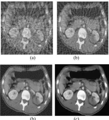
Comparison of reconstruction techniques such as BP, FBP (analytical), & Gradient and Bayesian algorithm (iterative) with respect to quality of reconstructed images is presented in this section. The reconstruction performances are calculated for 16, 32, 64 and 180 projections. The simulated results as well as Fig. 3 show that minimum 64 projections, with coverage angle ranging from 0 to 180º with an incremental value of 3º is necessary to reconstruct the image with acceptable quality.
(a) (b)
(c) (d)
Fig. 2. Reconstructed image of standard medical image by BP using (a)16, (b) 32, (c) 64 and (d) 180 projections.
This technique generates star or spoke artifact. Fig. 2 clearly reveals that the quality of reconstructed image increases as number of projections increases. However the reconstructed image appears to be very blurry. Fig. 3 shows reconstruction of the standard medical of abdomen by FBP with coverage angle ranging from 0 to 180º with an incremental value of 10º to 2º.
(a) (b)
(b) (c)
Fig. 3. Reconstructed image of the standard medical image, by FBP (with Sheep logan filter) using (a)16, (b) 32, (c) 64 and (d) 180 projections.
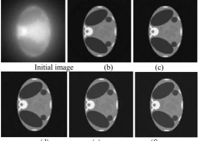
Fig. 3 clearly reveals that the quality of reconstructed images of the standard medical image of abdomen increases as number of projection increases, the errors df and dp of the reconstructed images remain constant after 32 projections. This algorithm requires minimum of about 32 projections with rotational increment of 50 to display acceptable reconstructed image. The resultant reconstructed images obtained from Gradient algorithm by varying the number of iterations, are shown in Fig. 4. The later demonstrates that Gradient algorithm is providing better reconstruction than that of FBP and BP. The quality measurements df and dp
Initial image (b) (c)
(d) (e) (f)
Fig. 4. Reconstructed images by Gradient algorithm using (b) 20, (c) 60, (d)100 (e) 200 and (f) 500 iterations
The experiments revealed major observations; as the number of projections within a given angular range was increased, the quality of reconstructed image appeared better for analytical and iterative algorithms. The errors df and
dp obtained from the Bayesian algorithm are less than those of BP, FBP and Gradient algorithms. Also, the star artifact appearing in image reconstructed from the filtered back projection is disappeared with the method of Gradient and Bayesian algorithms. It was found, for both analytical and iterative methods studied in this work that the quality measurements decreased with increasing number of projections. The number of iteration in the case of Gradient and Bayesian algorithms is much required in order to enhance the image quality.
VII. CONCLUSION
This paper presents the comparisons of the image reconstruction algorithms using BP, FBP analytical methods, Gradient and Bayesian algorithms. In this work, objective measurement by two relative norm errors of the resulting images and simulated projections, led to an ability to subjectively judge the reconstructed image quality. By Gradient and Bayesian algorithms, the problems in Star artifacts, the quality measurements and the reconstructed image quality can be improved significantly. The results show that Bayesian method provides the best image quality and small values of the errors df and dp . From the simulated results, we shall conclude that the Bayesian algorithm is reliable and practical to enhance the quality of reconstructed images for CT applications.
(a)
(b) Fig. 5. Relative norm errors v/s iterations for Gradient algorithm (a) (b)
Initial image (b) (c)
(d) (e) (f)
Fig. 6. Reconstructed images by Bayesian algorithm using (b) 20, (c) 60, (d)100 (e) 200 and (f) 500 iterations
ACKNOWLEDGMENT
We thank M.A Djafari for inspiring discussions and explanation of Bayesian theory during the short stay of Z. Messali in Supelec, France 2011.
REFERENCES
[1] Q. Zhong, W. Junhao, and Y. Pan, “Algebraic Reconstruction Technique in Image Reconstruction with Narrow Fan Beam,” IEEE. Trans. Medical Imaging, vol. 52, no. 5, pp. 1227-1235, Oct 2005. [2] ative Reconstruction Algorithmsin
SPECT,” Journal of nuclear medicine, vol. 43, no. 10, pp.1343–1358, Oct 2002.
[3] C. Soussen and A. M. Djafari, “Closed surface reconstructionin X-ray tomography,” in Proc. IEEE Int. Conf. Image Processing, vol. 1, pp. 718–721, Thessaloniki, Greece, Oct 2001.
[4] A. C. Kak and M. Slaney, “Principles of computerized tomographic imaging,” IEEE Press, pp. 92-93, 1988.
Zoubeida Messali received the B.Sc. and M.Sc.
degrees in electronic engineering from the University of Constantine, Constantine, Algeria, in 1995 and 2000, respectively, and the Ph.D. degree in electronic engineering from the University of Constantine, in 2007. From 1996 to 2001, she was a Tutor with the electronic engineering department, University of Constantine. From 2002 to 2007, she was a Lecturer at the electronic engineering department, University of M’Sila, Algeria. She is currently an associate Professor with the electronic department, University of Bordj Bou arreridj. Her current research interests include image processing, tomography reconstruction, electron tomography, denoising methods with wavelet, Bayesian approaches and multiresolution analysis.
Nabil Chetih received a received the B.Sc. degree in electronic engineering from the University of M'sila, Algeria, in 2008, the diploma magister degree in image and signal processing, in 2012 from the University of Sciences and Technology (USTHB) of Algiers, he has a member at L2TIR laboratory, in Department of Telecommunications, University of Sciences and Technology (USTHB). His main scientific interests include image processing, Computed Tomography (X-ray, PET, SPECT and eddy current imaging), image reconstruction ,Bayesian inference approaches for inverse problems in general, segmentation of the image , multiresolution image analysis.
Amina Serir Benmerabet received a magister
degree in image and signal processing, in 1991 and her PhD degree from the University of Sciences and Technology (USTHB) of Algiers, in 2002. Since 2000, she is the leader of the team “2D and 3D image processing” of the L2TIR laboratory, in Department of Telecommunications, University of Sciences and Technology (USTHB). Her scientific interests include image processing, compression, multiresolution and multidirectional image analysis and biometrics.
Abdelwahhab Boudjelal received the B.Sc.
and M.Sc. degrees in electronic engineering from the University of M'sila, M'sila, Algeria, in 2007 and 2010, respectively.
From 2008 to day, He was a Tutor with the electronic engineering department, University of M'sila. Since 2011, he has a member at “Laboratoire de Génie Electrique” (LGE) at Université de M’sila.
The main application domains of his interests are Computed Tomography (X-ray, PET, SPECT and eddy current imaging), image processing, Bayesian approaches and multiresolution analysis.