© Penerbit UTHM DOI: https://doi.org/10.30880/ijie.2018.10.06.005
Group Method of Data Handling with Artificial Bee Colony in
Combining Forecasts
Nurhaziyatul Adawiyah Yahya
1, Ruhaidah Samsudin
1, Irfan Darmawan
2, Ani
Shabri
3*, Shahreen Kasim
41
School of Computing, Faculty of Engineering,
Universiti Teknologi Malaysia, 81310 Johor Bahru, Johor, Malaysia.
2
School of Industrial Engineering, Telkom University, 40257 Bandung, West Java, Indonesia.
3
Mathematics Department, Faculty of Science
Universiti Teknologi Malaysia, 81310 Johor Bahru, Johor, Malaysia.
4
Faculty of Computer Science and Information Technology Universiti Tun Hussein Onn Malaysia, 86400, Johor, Malaysia.
Received 28 June 2018; accepted 5 August 2018, available online 24 August 2018
1. Introduction
Time series forecasting is an essential part in forecasting, used in various areas such as business, finance and engineering. In time series forecasting, similar variables from past observations are collected and analysed. From the analysis, a model which describes the underlying relationship between the input and output variables will be developed and will then be used to extend the time series into the future. This method is applicable when not much information on the underlying data generating process is available or when there is no suitable explanatory model that can map the prediction variable to other explanatory variables.
For decades, researchers have been studying and researching on ways to improve the forecasting accuracies [1, 2]. Numerous experimental studies suggested that the combination of several different models can improve the forecasting accuracies compared to individual model [3,4,6-9]. The concept of
combination of different models is simply to utilise the distinctive features of each individual models in learning different data patterns. Past literatures also observed that model combination is able to reduce the errors arising from faulty assumptions, bias, or mistakes in the data to a great extent. Therefore, using the combination method is the best option if there is a lot of uncertainty and issue in selecting the optimal forecasting model.
After the work of Bates and Granger was proposed in 1969 [12], several forecasts combination techniques have since been developed [13-15]. Amongst them are the weighted linear combinations, which is one of the most popular combining techniques due to its simplicity. In this technique, the weights of the individual model are either equal or be based on some mathematical rule. Other common forecasts combination methods are statistical methods for example the simple average and error-based method [16, 17].
Abstract: In this study, the use of Artificial Bee Colony (ABC) algorithm to combine several time series forecasts is presented. This study is done by combining individual forecasts of Group Method of Data Handling models using the weighted-based combine approach. The weights for each individual model are calculated using ABC algorithm. In order to evaluate the proposed model, this study tested the proposed model on the International Airline Passengers data, and the performances are calculated using mean square error (MSE), mean average error (MAE) and mean average percentage error (MAPE). The accuracy of the proposed model is compared to the individual models and the models implemented in previous literatures. The results revealed that the proposed model produced significantly accurate forecasts.
Recently, combination methods using optimization algorithms has been used in literatures such as by [18] which used Particle Swarm Optimization (PSO) and Genetic Algorithm (GA), [19] which used rule-based induction methods and [20] which proposed MLP neural networks to calculate appropriate weights for combination of several time series models. Nevertheless, compared to traditional statistical methods, the literatures on the usage of artificial intelligence method for forecast combination is still limited and require further research and development.
In this paper, a combination technique using Artificial Bee Colony (ABC) algorithm for finding appropriate weights to combine several Group Method of Data Handling (GMDH) models is proposed. This proposed technique is partially motivated by the work of Kondo et al. [21] which implemented three types of neural network architectures in GMDH to automatically organize the GMDH’s network architecture in medical imaging. In this paper, instead of implementing three types of architectures in one model, we propose forecasting several GMDH models, each using different types of neural network architectures. The appropriate combination weights are determined using ABC from the performances of the individual models on the validation datasets. This technique will utilise the strength of each individual model, without increasing the complexity of the computation. The effectiveness of this technique is tested using real-world time series data which is frequently used in previous literatures. Additionally, the performances of the proposed combined method are compared to the individual GMDH models and several models from previous researches.
The rest of the paper is organized as follows. In the next section, the combine approach, ABC algorithm in optimization, GMDH modelling approaches in forecasting are briefly reviewed. The proposed combined approaches will also be introduced in Section 2. In Section 3, empirical results from a real data set and a benchmarked data set are discussed, followed by the last section which contains the conclusion of this research.
2.
Methodology
2.1
Weighted-based Combine Approach
Based on past researches, various methods are available in combining forecasts. However, our focus in this research will be on the weighting-based combine approach. This widely accepted approach is done by giving a weight coefficient to each individual forecast based on its performance and then aggregate it. The formula for this approach is as follows:
( 1 )
Where is the weight of the nth individual model, and N is the total number of individual models to be combined. Meanwhile, is the forecasted value of the nth
individual model at H steps ahead, based on its performance at time T and is the result of the forecast combination at H steps ahead based on its performance at time T.
Additionally, in most literatures, constraints are imposed on the weights as follows:
( 2 )
Even though positive weights have been applied in numerous studies, in this research, we implemented the no negative constraint theory proposed by [18] whereby the negative weights are also taken into considerations.
2.2
ABC Optimization Algorithm
Artificial Bee Colony is a relatively new optimization algorithm proposed by Karaboga [22]. This algorithm was inspired by the behaviour of honey bees in foraging for food. Basically, this algorithm consists two types of foragers; employed foragers and unemployed foragers. Employed foragers consists of the employed bees (also known as recruited bees), while unemployed foragers consist of two types of bees; onlooker bees and scout bees.
In ABC algorithm, employed bees will carry information about the food sources (such as the position of food source from the nest) and share it with onlooker bees. This information represents a possible solution to the optimization problem. The onlooker bees will evaluate and choose the food source based on the quality of the nectar. This is done by calculating the probability of the fitness value using the formula in (3):
( 3 )
Where N is the number of food sources, and is the fitness value of solution j.
The employed bees whose food sources has been abandoned will then turn into a scout bee and search for a new solution. These steps are repeated until it reaches the maximum number of cycles.
The general steps in ABC is described as follows: Step 1: Initialize solutions.
Step 2: Repeat until stopping criteria is met:
- Send employed bees and calculate the fitness.
- Send onlooker bees and calculate the fitness.
- Send scout bees to look for another solution.
- Memorize best solution. Step 3: Stop.
2.3
GMDH Model
( 4 )
Where a represents the coefficients, x are the inputs variables, M is the number of input variables, and y is the output variable of the system. The equation in (4) can be accomplished by using a feed-forward self-organizing polynomial functional network.
The basic design procedure for GMDH is described below:
Step 1: For input variables X = {x1, x2, … xM}, where M is the total number of inputs, the dataset is first divided into training and testing sets. The training set is for the model construction, while the testing set is for the assessment of the model.
Step 2: In constructing the architecture of GMDH model, the training data are fed to the model two at a time. The number of combinations for each layer can be calculated using (5):
( 5 )
In conventional GMDH, each combination of input will form an input node that tries to model the system’s output by using polynomial as shown in (6) below:
( 6 )
The coefficients a, b, c, d, e and f in equation above is obtained by using regression.
Step 3: The performance of the inputs will be evaluated using RMSE, and based on a certain threshold, variables that performs the worse will be eliminated.
Step 4: Steps 2 to 3 are repeated in each layer until the stopping criterion is triggered. This happens when the performance of the last layer worsened.
Step 5: Once the GMDH structure has been established, the testing data will be input to the structure to produce a forecast.
2.4
Proposed Combined Method
In previous research by [21] and [24], it was shown that using several neuron architectures (or transfer functions) within a model produced better results than the model which only use one. Nevertheless, increasing the number of transfer functions in a model will increase the model’s complexity. Furthermore, it is quite inflexible for the modellers to add more transfer function in the future. Hence, this research proposed combining several GMDH models, each using only one transfer function. By doing this, the computation will be much simpler and more flexible. The steps for the proposed method are as follows:
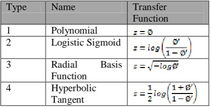
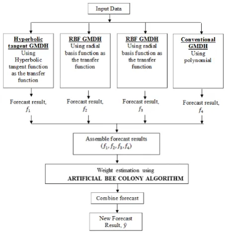
Step 1: The forecasting steps is similar to GMDH conventional model. However, in this proposed method, 4 GMDH models are developed, each using different types of transfer functions as shown in Table 1.
Table 1: Different types of transfer functions.
Type Name Transfer
Function 1 Polynomial
2 Logistic Sigmoid 3 Radial Basis
Function 4 Hyperbolic
Tangent
Step 2: For each combination of 2 inputs (for example, and ), can presented as shown in (6). For each transfer function, the values of are calculated as shown in Table 2.
Table 2: Values of Z for each transfer function.
Type Name Transfer
Function 1 Polynomial
2 Logistic Sigmoid
3 Radial Basis
Function 4 Hyperbolic
Tangent
Where is the output variable and is the normalized output variable.
Step 3: The generated forecasting output for each model can be written as , where N is the total number of models to be combined.
Step 4: In combining the forecasted output, the determination of the appropriate weights is depicted in matrix form below:
( 7 )
Step 5: In this study, ABC algorithm will estimate the weights for (7) by generating random weights at each iteration. Then the best weight is selected by calculating the performance of output using sum of squares error (SSE) in (8):
( 8 )
Where is the actual value and is the forecasted value. The process of finding suitable weights are repeated until ABC’s maximum cycle is reached.
Fig. 1: The overall process involved in the proposed method.
3.
Data
In this research, the reliability of the proposed model is tested on the well-known international airline passengers’ data. This data has been previously used by several researches in forecasting area and has a strong seasonal pattern. The airline data was taken from January 1949 to December 1960 (comprising of 144 total datasets), which comprises of the total number of passengers on international airlines in thousands. The division of the data in for the development of GMDH model in this research is 90% training, and 10% testing.
Fig. 2: International airline passengers time series (Jan 1949-Dec 1960).
4.
Performance Criteria
To assess the performance of the proposed model, mean squared error (MSE), mean absolute error (MAE) and mean absolute percentage error (MAPE) are used in this research. These three statistical measurements are
often used in the evaluating the performances of forecasting models [25]. The formula for these measurements are as follows:
( 9 )
( 10 )
( 11 )
Where is the sample size, is the actual value and is the forecasted value of the model. A model is considered the best if it has the smallest value of MSE, MAE and MAPE.
5.
Experiments and Results
In this study, the implementation of GMDH and ABC is done using MATLAB R2014b. The execution of ABC is simple, due to it having few numbers of parameters i.e. decision variables size, decision variables upper and lower boundaries and maximum number of iterations. The decision matrix size depends on the number of weights to be estimated (in this case, 1x4, whereby 4 is the number of individual models which is intended to be combined). The maximum and the minimum value of decision variables is set as 1 and -1 respectively, since this research considers the no negative constraint theory. The cost function used in this study is SSE. SSE will calculate the performance of weights which are randomly generated by ABC at each iteration. Weights which produced the smallest SSE will be kept at each cycle, and by the end of the iterations, the best weights will be presented. These weights will then be used to combine each individual model as explained in the previous sections. In this study, the maximum number of iterations for ABC is 50.
The output for the forecasting of the individual models and the proposed combined GMDH model is depicted in Fig. 3.
Table 3: Comparing the performance of the proposed model with individual models.
Models MSE RMSE MAE MAPE
Individ-ual Models
Convent -ional
244.45 15.63 12.13 2.69
RBF 1987.19 44.58 26.08 5.03 Sigmoid 861.94 29.36 25.54 5.32 Tanh 249.35 15.79 12.58 2.79 Combined Model 139.76 11.82 9.85 2.27
Table 3 shows the performances of individual GMDH models and the proposed combined model. Based on the results of the individual models, it can be seen that the forecasting results varies depending on the type of transfer functions used. Among the four models, GMDH which used radial basis function (RBF) performed the worst in terms of MSE, with a value of 1987.19. This is a very large value when compared with the conventional GMDH (which used polynomial transfer function). The same can be said about GMDH which utilized logistic sigmoid transfer function, with MSE of 861.94. On the other hand, the conventional GMDH performs the best among the four models, followed by GMDH using hyperbolic tangent transfer function with MSE of 244.45 and 249.35 respectively. This indicates the possibility that GMDH using RBF and logistic sigmoid transfer function could not properly capture the seasonal patterns of the international airline passenger’s data.
The empirical results also demonstrate that by combining the models, a better result can be obtained even though the performances of the individual models vary by a large margin. In the table shown, the proposed combined model managed to further reduce the MSE value of the best individual model by 57%. This result is consistent with the theory of forecast combination, whereby the strengths of each single model are being exploited. Furthermore, the heuristic nature of ABC which generates random weights at each iteration enable the best weights to be discovered unlike the traditional statistical method which is static.
Table 4: Comparing the performances of the proposed model with models from previous literatures.
Model MSE
Faraway’ ARIMA (1987) 325.839
Faraway’ ANN (1987) 241.670
Samsudin et al.’s GLSSVM (2011) 228.546
Proposed Combined GMDH 139.7649
To further assess the proposed model, the models previously used in past literatures are used to compare the performances. These models also applied international airline data, making it suitable to be used as benchmark models. As shown in Table 4, the proposed model is compared to a linear model and 2 non-linear models from past literatures. The models consist of the notable ANN and ARIMA model which was modelled by [26], and
GLSSVM model which was proposed by [27-28]. The results showed that the linear model, ARIMA produced the worst result with MSE of 325.839 followed by ANN with MSE of 241.670. This result proved that ARIMA has failed to completely capture the non-linearity of the airline data due to it being a linear model. ANN on the other hand is a non-linear model, and hence have a better chance in capturing the underlying patterns in the data.
However, GLSSVM model performed better than both ARIMA and ANN, with MSE of 228.546. This is mainly because GLSSVM is a combination of two models; GMDH with least squares support vector machine (LSSVM) model. A hybrid model usually has the tendency to outperform a single individual model. However, hybridization is usually done using two or three individual models. If more individual models are included, the model will become too complex [18]. Conversely, a combination method can combine large amount of individual models without having computation difficulties. Furthermore, the more individual models are combined, the better the forecast output as seen in the work of [18]. Thus, the proposed model in this study managed to produce a result which is significantly better than the three benchmark models with MSE of 139.76.
6.
Summary
It is a well-known fact in the forecasting area that there is no model that can perform well for all types of data. Real world data are usually a mix of linear and non-linear, and often have different characteristic from one another. That is to say, even if a model performs well for a certain data, it might not be able to perform best in another data. One of the best way to solve this issue is by combining the models so that the strength of each model could be utilize. In this study, we proposed combining several heuristic GMDH models (each modified with different transfer functions) using ABC algorithm on a seasonal time series data. We have demonstrated that by combining the models using ABC, the results could be better improved even though the performances of each model differ from one another. This is due to the fact that ABC algorithm is heuristic in nature and is able to discover the best weights for each individual model. Hence, the empirical results from this study prove that ABC algorithm can be a promising tool for combining time series data.
References
[1] De Gooijer, J.G. and Hyndman, R.J., 2006. 25 years of time series forecasting. International journal of forecasting, 22(3), pp.443-473.
[2] Box, G.E. and Jenkis, G.M., 1970. Time series analysis for casting and control (No. 519.232 B6). [3] Armstrong, J.S., 2001. Combining forecasts.
[4] Zhang, G.P., 2003. Time series forecasting using a hybrid ARIMA and neural network model. Neurocomputing, 50, pp.159-175.
[5] Makridakis, S., Andersen, A., Carbone, R., Fildes, R., Hibon, M., Lewandowski, R., Newton, J., Parzen, E. and Winkler, R., 1982. The accuracy of extrapolation (time series) methods: Results of a forecasting competition. Journal of forecasting, 1(2), pp.111-153.
[6] Makridakis, S., 1989. Why combining works?. International Journal of Forecasting, 5(4), pp.601-603.
[7] Newbold, P. and Granger, C.W., 1974. Experience with forecasting univariate time series and the combination of forecasts. Journal of the Royal Statistical Society. Series A (General), pp.131-165. [8] Palm, F.C. and Zellner, A., 1992. To combine or not
to combine? Issues of combining forecasts. Journal of Forecasting, 11(8), pp.687-701.
[9] Winkler, R.L., 1989. Combining forecasts: A philosophical basis and some current issues. International Journal of Forecasting, 5(4), pp.605-609.
[10] Clemen, R.T., 1989. Combining forecasts: A review and annotated bibliography. International journal of forecasting, 5(4), pp.559-583.
[11] Makridakis, S., Chatfield, C., Hibon, M., Lawrence, M., Mills, T., Ord, K. and Simmons, L.F., 1993. The M2-competition: A real-time judgmentally based forecasting study. International Journal of Forecasting, 9(1), pp.5-22.
[12] Bates, J.M. and Granger, C.W., 1969. The combination of forecasts. Journal of the Operational Research Society, 20(4), pp.451-468.
[13] Clemen, R.T., 1989. Combining forecasts: A review and annotated bibliography. International journal of forecasting, 5(4), pp.559-583.
[14] Aksu, C. and Gunter, S.I., 1992. An empirical analysis of the accuracy of SA, OLS, ERLS and NRLS combination forecasts. International Journal of Forecasting, 8(1), pp.27-43.
[15] Zou, H. and Yang, Y., 2004. Combining time series models for forecasting. International journal of Forecasting, 20(1), pp.69-84.
[16] Jose, V.R.R. and Winkler, R.L., 2008. Simple robust averages of forecasts: Some empirical results. International Journal of Forecasting, 24(1), pp.163-169.
[17] Lemke, C. and Gabrys, B., 2010. Meta-learning for time series forecasting and forecast
combination. Neurocomputing, 73(10-12), pp.2006-2016.
[18] Xiao, L., Wang, J., Dong, Y. and Wu, J., 2015. Combined forecasting models for wind energy forecasting: A case study in China. Renewable and Sustainable Energy Reviews, 44, pp.271-288.
[19] Arinze, B., Kim, S.L. and Anandarajan, M., 1997. Combining and selecting forecasting models using rule based induction. Computers & operations research, 24(5), pp.423-433.
[20] Prudêncio, R. and Ludermir, T., 2004, December. Using machine learning techniques to combine forecasting methods. In Australasian Joint Conference on Artificial Intelligence (pp. 1122-1127). Springer, Berlin, Heidelberg.
[21] Kondo, T., Ueno, J. and Takao, S., 2012, December. Hybrid multi-layered GMDH-type neural network using principal component-regression analysis and its application to medical image diagnosis of lung cancer. In BioMedical Computing (BioMedCom), 2012 ASE/IEEE International Conference on(pp. 20-27). IEEE.
[22] Karaboga, D., 2005. An idea based on honey bee swarm for numerical optimization (Vol. 200). Technical report-tr06, Erciyes university, engineering faculty, computer engineering department.
[23] Farlow, S.J., 1981. The GMDH algorithm of Ivakhnenko. The American Statistician, 35(4), pp.210-215.
[24] Taušer, J. and Buryan, P., 2011. Exchange Rate Predictions in International Financial Management by Enhanced GMDH Algorithm. Prague Economic Papers, 20(3), pp.232-249.
[25] Zhang, G., Patuwo, B.E. and Hu, M.Y., 1998. Forecasting with artificial neural networks: The state of the art. International journal of forecasting, 14(1), pp.35-62.
[26] Faraway, J. and Chatfield, C., 1998. Time series forecasting with neural networks: a comparative study using the airline data. Journal of the Royal Statistical Society: Series C (Applied Statistics), 47(2), pp.231-250.
[27] Samsudin, R., Saad, P. and Shabri, A., 2011. A hybrid GMDH and least squares support vector machines in time series forecasting. Neural Network World, 21(3), p.251.