17
Synchronous Pendulums and
Aliasing
J. C. Chong1,2, W. F. Chong , H. H. Ley2
1
Adv. Photonics Science Institute, Universiti Teknologi Malaysia, 81310, Skudai, Johor.
2
Dept. of Physics, Faculty of Science, Universiti Teknologi Malaysia, 81310, Skudai, Johor.
*Corresponding email: [email protected]
Abstract
We present the construction, mathematical relation and simulation of a 16-bob pendulum wave machine (PWM). Following small angle approximation, the PWM is a useful teaching aid to demonstrate free oscillations and periodic motion; it can also illustrate effects of aliasing in physics and engineering. The duration of pattern cycle is adjusted with a set of pendulum lengths that are dictated by a non-linear function followed by the outline of the PWM design aspects.
18
1. INTRODUCTION
First built by Ernst Mach around 1687 to demonstrate synchronized oscillation, the pendulum wave machine was designed as a university level teaching-aid. It composed of a series of pendulum with increasing bob length following a specific function. When released simultaneously, each pendulum oscillates with a slightly different period from the next, resolving a fascinating display of patterns resembling travelling waves, standing waves, beating and random motion. The PWM has been and is still being used in lecture halls to demonstrate important concepts in classical physics such as potential and kinetic energy in mechanics, gravitational potential, air resistance, mechanical friction, and aliasing in signal processing.
2. MATHEMATICAL TREATMENT
The phenomenological equation describing the motion of the pendulum wave is derived based on the concept of simple harmonic equation where the small angle approximation are presumed and the damping due to air resistance, friction about pivot points and the elasticity of the string are not considered for simplicity. Consider the collective motion of the bobs such that it approximates the basic travelling wave equation as a function of distance x and time t given by equation (1);
) cos(
) ,
(x t A kxt
y (1)
where A is the amplitude, is the wave number, is the angular frequency and is
the phase angle. The wave number and angular frequency are related to the spatial and temporal information of the wave, that is the wavelength and period T as
and . As we displace the bobs by pulling them evenly to one
side, we define the moment prior to release as the beginning of series of oscillations where t = 0. At this moment, all pendulum locations defined by specific values of x, (we arbitrarily pick the first bob where x = 0) have maximum amplitude, A. Hence, by equation (1):
] ) 0 ( ) 0 cos[( )
0 , 0
( a k
y (2)
The initial condition requires the phase angle between the pendula to be zero, or physically it means the pendulum bobs are in the same position with respect to one another.
0 )
cos(
A
A
Now, as the time progresses, the collective wave pattern changes “shape” during its course of oscillation suggesting its wavelength is a function of time. Similarly, the period of oscillation for the pendulum bobs progressively increases against their position, x. Therefore, we can express both the wave number and angular frequency of the wave equation as a function of time and position respectively, i.e. k(t) and ω(x). Replacing these functions to equation (1) gives:
] ) ( ) ( cos[ )
,
(x t A k t x x t
19
From equation (4) k(t) and ω(x) are dependent on each other through parameter t and x. More specifically, it is due to our control of period, T for adjacent pendulum of increasing x, giving rise to the function of k(t). By describing the initial condition of the wave at t0 for t = 0 or x0 for x = 0 leads the wave equation into two general expressions:
] cos[
) ,
(x t A k0x 0t
y (5.1)
] ) ( cos[ ) ,
(x t A k t x 0t
y (5.2)
where the constants t0 and x0 helped to eliminate functions k(t) or ω(x) for one another, thus simplifying our work to model the wave pattern by choosing either (both equally valid) equation 5.1 or 5.2. Arbitrarily, consider equation 5.1, substituting t = 0 for initial condition when all pendulums are at maximum amplitude A; 0 ] 0 ) ( cos[ ) 0 ,
(x A A k0x x k0
y (6)
The oscillation of the pendulum wave pattern repeats itself where all the bobs return to its initial position after an interval of time. This period of time is defined as Tp which requires N number of oscillations for the first, longest pendulum (i.e. n=0) to complete one cycle of the wave patterns. Hence, its period T0 is given as:
N T
T0 p (7)
Observing the phase differences between pendula, the period of each pendulum
differs from its longer adjacent pendulum by exactly one oscillation per Tp cycle.
Hence, for T1, T2, T3 and so on, equation (7) can be generalized into:
n N
T Tn p
(8)
Applying the results of equation (8) into the definition of angular frequency earlier yields; p n T n N T
n) 2 2 ( )
(
(9)
Redefining x as the distance of any nth-pendulum away from the first (longest) pendulum, i.e. x = nd, where d is the common spacing between adjacent pendulums. Substituting x = nd into equation (9) eliminates the n parameter, leaving the angular frequency as:
p dT
x Nd x) 2 ( )
(
(10)
Substituting equation (10) to equation (6) followed by a few algebraic rearrangement results in the travelling wave equation that describes the “pendulum wave” pattern which is an expression of equation (5.2).
t T N x dT t A t x y p p 2 2 cos ) ,
20
2.1 Design of the Pendulum Wave Machine
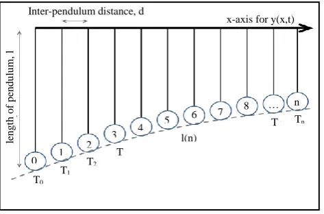
The mathematical treatment earlier does not provide information on certain design aspects in making a Wave Machine. The crucial information it ignored is the set of pendulum lengths that the machine needs to display those beautiful patterns. Fortunately, by assuming all pendulums oscillate freely in simple harmonic motion, a function, l(n) to describe the pendulum lengths with respect to its position on the x-axis can be formulated.
Figure 1: Pendula Configuration of the Wave Machine
In figure (1) the set of pendulums has a non-linear decreasing order of lengths against increasing y. This is because the difference between the oscillating period T, for each pendulum is directly proportional to the square root of its length, l. More specifically:
g l
T 2 (13)
where g is the standard gravity acceleration, 9.81 ms-2. By substituting equation (13) to the expression of angular frequency in equation (1) will arrive at the angular frequency for each pendulum with respect to its length. Because the length of pendulum changes for different pendulum bobs, both the angular frequency and pendulum length can be expressed as a function of n.
) ( ) (
n l
g n
(14)
Substituting equation (14) to equation (9) for eliminating ω(n) and by rearranging to give the expression for the length of pendulum l(n) as;
2
) ( 2 )
(
n N T g n
l p
(15)
Inter-pendulum distance, d
x-axis for y(x,t)
le
n
g
th
o
f
p
en
d
u
lu
m,
l
0 1
2 3
4 5
6 7 8 …
T0
n
l(n)
T
T1 T2
T 3
21
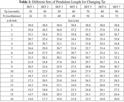
From equation (15), the series of pendulum length to display the wave pattern can be determined by assigning two parameters: the time it takes for the pendulum wave pattern to repeat itself, Tp, and the number of oscillations, N it takes for the longest pendulum (n=0) to reach Tp.
Table 1: Different Sets of Pendulum Length for Changing Tp
SET 1 SET 2 SET 3 SET 4 SET 5 SET 6 SET 7
Tp [seconds] 30 40 50 60 70 80 90
N [oscillations] 24 32 40 48 56 64 72
n-th bob l(n) [cm]
0 38.8 38.8 38.8 38.8 38.8 38.8 38.8
1 35.8 36.5 36.9 37.2 37.5 37.6 37.8
2 33.1 34.4 35.2 35.8 36.2 36.5 36.7
3 30.7 32.4 33.6 34.4 35.0 35.4 35.8
4 28.5 30.7 32.1 33.1 33.8 34.4 34.8
5 26.6 29.0 30.7 31.8 32.7 33.4 33.9
6 24.8 27.5 29.3 30.7 31.7 32.4 33.1
7 23.3 26.1 28.1 29.6 30.7 31.5 32.2
8 21.8 24.8 27.0 28.5 29.7 30.7 31.4
9 20.5 23.6 25.9 27.5 28.8 29.8 30.7
10 19.3 22.5 24.8 26.6 27.9 29.0 29.9
11 18.3 21.5 23.9 25.7 27.1 28.3 29.2
12 17.3 20.5 23.0 24.8 26.3 27.5 28.5
13 16.3 19.6 22.1 24.0 25.6 26.8 27.8
14 15.5 18.8 21.3 23.3 24.8 26.1 27.2
15 14.7 18.0 20.5 22.5 24.1 25.5 26.6
16 14.0 17.3 19.8 21.8 23.5 24.8 26.0
22
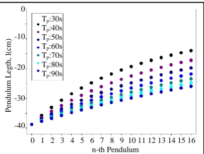
Figure 2: Pendulum Bob Positions for Different Sets of Tp
Figure (2) shows sagittal view of our Wave Machine with points showing individual pendulum bobs with different Tp. It shows shorter Tp results an overall decrease of pendula length. This is a significant consideration towards the design of an efficient pendulum wave machine. Ideally, the machine is best to exhibit at least one complete cycle of the travelling wave pattern, Tp before the pendula start to lose energy. The trend suggest using pendulum lengths with shorter Tp, where upon release, the pendula will have enough initial potential energy to oscillate until the entire sequence of travelling wave pattern repeats itself.
However, the shorter pendulum length will result in higher angle of release which changes the oscillation of the pendulum from simple harmonic motion to non-linear oscillation [4,5] thus lowering its temporal periodicity i.e. the bob lost its synchrony between each swing with respect to one another. By using longer pendulum lengths, the problem with initial angle of release is reduced but in exchange it takes longer time to complete one travelling wave cycle and the limiting case becomes the initial potential energy such that damping will be contribute to distort and prevent the pendulum wave from completing the pattern.
Notice as Tp was set to 30 seconds, the shortest pendulum (n=16) will be dangling at merely 14 centimetres from the pivot. Although this significantly increased the repetition of oscillation it also reduced the small angle approximation which was a crucial assumption made earlier in the mathematical treatment.
0 1 2 3 4 5 6 7 8 9 10 11 12 13 14 15 16 n-th Pendulum
0
-10
-20
-30
-40
P
en
d
u
lu
m L
eg
th
,
l(
cm)
23
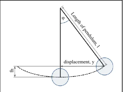
Figure 3: Free Oscillation Diagram of Single Pendulum
As mentioned earlier, regularity of pendulum oscillation comes from small angle approximation – the existence of a maximum initial angle of release of the pendulum bobs for equation (13) to be valid. Since all pendulum bobs are equally displaced from initial y-axis, shorter pendula have larger angle of release compared to longer ones. Referring to figure (3) where the lengths and release angle of a simple pendulum are illustrated; notice that dl have to be as small as possible. As a consequence, both angle and y-axis displacement have to be as small as possible. The degree of approximation based on the sets of pendulum lengths are tabulated in table (2) by sampling the small angle approximation on the shortest pendulum bob (n=16). By displacing the bobs to an initial amplitude (+Y in centimetres) its cos(φ) is evaluated.
Table 2: Asymptotic Approximation for cos (φ) such that φ=1
SET 1 SET 2 SET 3 SET 4 SET 5 SET 6 SET 7
Tp [seconds] 30 40 50 60 70 80 90
N [oscillations] 24 32 40 48 56 64 72
+Y [cm] cos (φ) for pendulum bob n = 16
1 0.9974 0.9983 0.9987 0.9990 0.9991 0.9992 0.9993
2 0.9897 0.9933 0.9949 0.9958 0.9964 0.9968 0.9970
3 0.9767 0.9848 0.9885 0.9905 0.9918 0.9927 0.9933
4 0.9581 0.9727 0.9794 0.9831 0.9854 0.9870 0.9881
5 0.9338 0.9571 0.9676 0.9734 0.9771 0.9795 0.9813
Table (2) shows that even at Tp set to 30 seconds where its shortest pendulum only 14 cm from the pivot approximates fairly well to the trigonometric function provided the initial displacement no more than 5 cm away from the centre. Experimentally, displacement of about 5 cm provides enough gravitational potential energy for the pendulum to oscillate for about a minute without losing too much
displacement, y
dl
24
energy to dampening sources such as pivotal friction and air resistance. Since oscillation of the pendulum was experimentally found to be limited by dampening mechanism to about 60 seconds, only pendula lengths from SET 1 to SET 4 is applicable.
2.2 Travelling Wave Function Plot
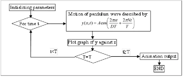
A time-evolution of the pendulum wave is plotted in MATLAB using any provided input values such as inter-pendulum distance, d period of travelling wave, Tp and the number of oscillations, N needed for the longest bob to complete one cycle of wave patterns, Tp. By fixing these parameters according to the actual design of the Wave Machine, where d = 0.032 meter, N = 48 and Tp = 60 seconds, the linear computation algorithm used is illustrated in figure (4).
The resulting numeral data are then graphically visualized, showing how the Wave Machine looks like from top-down perspective where blue line indicates travelling wave function while black dots represent individual pendulum bobs where the “snapshots” of the Wave Machine at specific intervals are shown in figure (5) and the wave pattern from the PWM constructed is illustrated in figure (6). Each of these pattern repeats itself within one cycle of Tp starting t = 0, symmetrical at t = (1/2)Tp, where every adjacent pendulum have maximum phase difference.
Figure 4: Computation algorithm for pendulum wave simulation
25
Figure 5: Simulation of pendulum motion and travelling wave function on the wave
machine
Figure 6: Travelling wave snapshot at different time from the constructed PWM,
starting from top left and ends at lower right, shows the wavelength decreases with time.
Pendulum Wave Machine Simulation Pendulum Wave Machine Simulation Pendulum Wave Machine Simulation
0 0.1 0.2 0.3 0.4 0.5 0.6 x-axis (metre)
Pendulum Wave Machine Simulation
0 0.1 0.2 0.3 0.4 0.5 0.6
x-axis (metre) 0 0.1 0.2 0.3 0.4 0.5 0.6 x-axis (metre) Pendulum Wave Machine Simulation Pendulum Wave Machine Simulation
0.06 0.04 0.02 0 -0.02 -0.04 -0.06 0.06 0.04 0.02 0 -0.02 -0.04 -0.06 0.06 0.04 0.02 0 -0.02 -0.04 -0.06 Am p li tude ( m et re ) Am p li tude ( m et re ) Am p li tude ( m et re )
0 0.1 0.2 0.3 0.4 0.5 0.6
x-axis (metre) 0 0.1 0.2 0.3 0.4 0.5 0.6 x-axis (metre) 0 0.1 0.2 0.3 0.4 0.5 0.6 x-axis (metre) Pendulum Wave Machine Simulation Pendulum Wave Machine Simulation Pendulum Wave Machine Simulation
0.06 0.04 0.02 0 -0.02 -0.04 -0.06 0.06 0.04 0.02 0 -0.02 -0.04 -0.06 0.06 0.04 0.02 0 -0.02 -0.04 -0.06 Am p li tude ( m et re ) Am p li tude ( m et re ) Am p li tude ( m et re )
0 0.1 0.2 0.3 0.4 0.5 0.6 x-axis (metre)
0 0.1 0.2 0.3 0.4 0.5 0.6 x-axis (metre)
26
The simulation shows the wavelength of the travelling wave function (blue line) shortens as time progresses. This imaginary blue line shows an “alternate pattern” effect is known as aliasing.
2.3 Aliasing
In short, aliasing is the emergence of two indistinguishable signals (aliases of one another) created by the sampling rate. Imagine a spinning disc with a black dot on its edge, completing one revolution per minute clockwise, its angular frequency at 1 rev/min is observable from the motion of the black dot. However if the snapshot of the black dot is taken once every 30 seconds; based on this new information it becomes difficult to distinguish the direction of disc rotation. Furthermore, if we observe the dot once every 75 seconds, the apparent motion of the black dot shows as if the disk is rotating in the counter clockwise direction.
The act of observing the disc at specific intervals of time is called sampling. For this case, sampling once every 30 seconds is the limit where its information produces ambiguous interpretation. When analogue signals such as flashing lights, rotating disc or sound beats are being sampled and recorded at specific rates (i.e. digitized), any component of the recorded signal above half of the analogue’s frequency will be aliased. Using our example, sampling once per 30 second is exactly half of the disc’s angular frequency, this limit is called the Nyquist frequency and it is one of the fundamental principles in understanding digital data acquisition.
An example of aliasing occurs when taking pictures of an object with periodic structure. A camera sensor has arrays of tiny pixels, but if it is not at least twice as dense as the periodic structure of the object will result in a type of aliasing known as spatial aliasing. The resulting image looks like a Moiré pattern. For an illustrative example, consider an object with a periodic structure such as a brick wall. From afar, the image of each brick is smaller than the pixel on the sensor; the details of individual bricks cannot be resolved unless the pixels are smaller. This result in the emergence of new pattern based on unresolved images where instead of flat even-coloured bricks, a colourful or black-and-white stripes are produced on the image of the wall.
27
Figure 7: Visual explanation of spatial aliasing in digital cameras [6]
The red crosses on the blue line are the reasons for spatial aliasing. Each cross indicates a location of sampling (individual pixels) and in this case the image is under-sampled which in turn creates a new false image as shown in the bottommost plot. Spatial aliasing is relatively easy to remove compared to temporal aliasing. Camera manufacturers usually add a low-pass filter in front of the camera sensor to “blur-out” very fine details in images that are comparable to the pixel dimensions that causes aliasing.
3. CONCLUSION
The mathematical treatment of the pendulum wave motion is outlined in a simple approach that is easy to grasp by undergraduates or pre-university physics students. The design of the pendulum wave machine is simple and thus suitable for demonstration purpose in lectures or classroom. Slight modification of this work would allow this topic to serve as a laboratory practical for introducing the concept of signal processing to students particularly the phenomenon of aliasing.
0 pi 0 pi 0 pi 0 pi Spatial Frequency Sinusoidal Respons
0 pi 0 pi 0 pi 0 pi Lens Interpreted: Spatial Response
0 pi 0 pi 0 pi 0 pi Sinusoidal Respons to Sampeled Response
0 pi 0 pi 0 pi 0 pi Sensor Pixel Interpreted Sampled Response 1
0.8 0.6 0.4 0.2 0
1 0.8 0.6 0.4 0.2 0
1 0.8 0.6 0.4 0.2 0
28
REFERENCES
[1] Harvard Natural Sciences Lecture Demonstrations, “Pendulum Waves -
Simple Harmonic and Non-Harmonic Motion”,
http://sciencedemonstrations.fas.harvard.edu/icb/icb.do, extracted on May 2014.
[2] J. H. Eberly, N. B. Narozhny and J. J. Sanchez-Mondragon, “Periodic
Spontaneous Collapse and Revival in a Simple Quantum Model”, Phys. Rev. Lett., Vol. 44, pp.1323, May 1980.
[3] Z. Gaeta, Ć. Dači, C. R. Stroud, “Classical and Quantum-mechanical
Dynamics of a Quasiclassical State of the Hydrogen Atom”, Phys. Rev. A., Vol.42, pp. 6308, Dec 1990.
[4] L. E. Millet, “The Large Angle Pendulum Period”, The Physics Teacher,
Vol. 41, pp.162, Mar 2003.
[5] R. B. Kidd, S. L. Fogg, “A Simple Formula for the Large-angle Pendulum
Period”, The Physics Teacher, Vol. 40, pp. 83, Feb 2002.
[6] B. Tobey, “Nikon D800E Overview: No Anti-aliasing Filter”,

![Figure 7: Visual explanation of spatial aliasing in digital cameras [6]](https://thumb-us.123doks.com/thumbv2/123dok_us/8443529.1702303/11.595.139.468.110.414/figure-visual-explanation-of-spatial-aliasing-digital-cameras.webp)
