Effect of Ambipolar Diffusion on the Flow of a Two-Component Plasma Gas Model in the Earth’s Planetary Ionosphere

http://www.sciencepublishinggroup.com/j/ijass doi: 10.11648/j.ijass.20170503.12

ISSN: 2376-7014 (Print); ISSN: 2376-7022 (Online)

Effect of Ambipolar Diffusion on the Flow of a

Two-Component Plasma Gas Model in the Earth’s Planetary

Ionosphere

B. S. Tuduo

*

, T. M. Abbey

Applied Mathematics and Theoretical Physics Group, Department of Physics, University of Port Harcourt, Port Harcourt, Nigeria

Email address:

[email protected] (B. S. Tuduo), [email protected] (T. M. Abbey) *_{Corresponding author}

To cite this article:

B. S. Tuduo, T. M. Abbey. Effect of Ambipolar Diffusion on the Flow of a Two-Component Plasma Gas Model in the Earth’s Planetary Ionosphere. International Journal of Astrophysics and Space Science. Vol. 5, No. 3, 2017, pp. 47-54. doi: 10.11648/j.ijass.20170503.12 Received: December 23, 2016; Accepted: January 5, 2017; Published: August 22, 2017

Abstract:

The paper presents analytical study on the effect of ambipolar diffusion on the flow of a two-component plasma gas in the Earth’s Planetary Ionosphere as a model to examine the ions-neutral and electrons-neutral atom interactions. The problem which consists of a set of partial non-linear differential equations was addressed using a plane wave and perturbation method of solutions. The result indicates that plasma frequency and electron-density in the Ionosphere increase with increase in magnetic field strength as well as with radiation and free convection parameters. It is observed that for;

the plasma interactive state becomes more stable, otherwise some bit of oscillation is noticed. The stability is seen to depend on the magnetic (M2_{) and thermal convection (G}

r) parameters. Under this condition the signal propagation becomes less diffuse

when the frequency of the signal is far greater than the plasma frequency, that is, ω >> p. The study aids our understanding of the effect of coupling frequency on the propagation of satellite signals through the ionosphere.

Keywords:

Ambipolar Diffusion, Two-Component Plasma Flow, Planetary Ionosphere

1. Introduction

The study of the ionosphere and its characteristics are important for both practical and scientific purposes; significantly due to its influence on the propagation of electromagnetic waves. Its studies date back to the pioneer work of Gughelmo Marconi, who successfully transmitted radio signal across the transatlantic on the 12th of December, 1901 [1, 2]. Today, the understanding of the chemical and dynamical processes of the ionospheric and astrophysical plasma has found applications in the areas of condensed matter Physics, nuclear Physics, thin panel displays (plasma TV), particle accelerators and communication, just to mention but a few. The ionosphere, which is the ionized part of the Earth’s upper atmosphere lies between the 60 and 1000 km, is known to be stratified into D, E, F1 and F2 layers respectively [3 - 5]. The solar extreme ultraviolent (EUV) and x-ray radiations as well as other cosmic radiations account for the ionization of the ionosphere [6 - 9], with the

D-layer being the lest ionized.

diffusion is prevalent in the core of molecular clouds which is a key factor in star formation (especially in the transfer of mass and momentum [19]), and the transfer and dissipation of energy in the Sun’s chromosphere [10].

Several researchers in the literature have extensively used numerical methods in the study of partially ionized plasma within the frame of single- or two-fluid models [20 - 26]. For example, [20] used semi-implicit scheme for two-fluid ambipolar diffusion to investigate instability in steady-state continuous shocks, while [21] described an explicit method for single-fluid ambipolar diffusion in the strong coupling limit. But, [27] investigated the heating through ambipolar diffusion in turbulent molecular clouds using a single-fluid approximation. Numerical schemes for the multi-fluid treatment of hall diffusion and ambipolar diffusion have been suggested by [28 – 30]. Whereas, [31] and [32] studied the properties of turbulence with ambipolar diffusion in a two-fluid approximation using three-dimensional (3D) numerical simulations model. Similarly, [26] presented a semi-implicit method for ambipolar diffusion using a two-fluid approximation. A fully explicit method for incorporating the single-fluid ambipolar diffusion into a multi-dimensional magnetohydrodynamic (MHD) code based on the total variation diminishing (TVD) scheme was described by [14]. While, [15] conducted a three-dimensional (3D) local sharing-box simulations to explore the effect of ambipolar diffusion on the non-linear evolution of magnetorotational instability (MRI) in the strong coupling limit. And just recently, [33] studied the dynamics of the interactions of neutrals and charged plasma particles in a single-fluid, ideal

magnetohydrodynamic framework to describe the

propagation of low-frequency waves in the partially ionized collision-dominated lower Earth’s Ionosphere, and the ionosphere-magnetosphere coupling.

In all the above studies, the effect of temperature differentials with accompanied radiative heat transfer and free convection motion; which is paramount in astrophysical regions where high temperature are experienced was not considered. This is the crux of this present study.

The paper is organized in the following format: - In section 2, the physics and the mathematical formulation of the problem leading to equation of motion shall be presented, while section 3 has the method of analysis leading to the derivation of different wave-modes and the attendant effects on the electrons and ions density variation in the ionosphere. Section 4 on the other hand discusses the various results and section 5 presents the conclusion. The study will aid our understanding of the chemical and dynamical processes of the ionosphere. It would further shed a light on the physics and factors affecting navigational satellites and global positioning systems.

2. Problem Formulations

In most regions of the ionosphere, particularly in the D-layer and some part of E-D-layer, ionization is seen to be weak. In this case the region is permeated with neutral gas

molecules along with ions and electrons. According to [15] in weakly ionized plasma, where ambipolar diffusion occurs as a result of the relative motion of the ions and neutrals, the inertia of the ionized species is usually negligible. It follows, therefore, that the ion velocity can be determined by the balance between the Lorentz force and ion-neutral gas collisional drag. It is this force balance along with other factors that determined and predict the motion of such an interacting system. If, therefore, V, B, P,

g

and are respectively the velocity field vector, magnetic field vector, the plasma pressure, the gravitational field vector and the density of the plasma component species; while qr is the

radiation flux resulting from the interaction of the cosmic and x-rays from the solar body on the Earth’s ionosphere; σ, the Stefan Boltzmann constant; α, the plasma optical property; T, the temperature of the medium and K0, χ , Cp, µ and e are the

thermal conductivity, porosity, specific heat capacity at constant pressure, neutral gas viscosity and electron charge, f , the coupling frequency between the ionized species and the neutral gas, whereas J is the current density, then the mathematical statements governing the flow of the two-component plasma model in the present of ambipolar diffusion are as follows;

= Q - L - ( ) (1)

= - + µ 2 +

g

+ (E + ) + ± ( - ) (2)

Cp = 2 - (3)

2 - 3 α2 - 16σα 2 = 0 (4)

x E = - !", (5)

x = # + $% J, (6)

∙ E = 4( ()* _{+ +} + ), ), (7)

∙ = 0 (8)

and J = ()* _{+ +}+ ), ) (9)

On the other hand, equation (2) shows, the force balance of the plasma within the ionosphere, the term is the force due to the pressure gradient, whereas the present of ρ_. g,

(E + ) and ( - ) {k ≠ n} terms indicate forces

due to gravity, electromagnetic fields and collision (or friction) between the ions (i) and the neutrals (n) with being the collisional frequency.

Also, equation (3) is the energy conservation equation, which indicates the present of 2 , the heat conduction term and , the heat absorption and transfer term. As we can readily see from equations (1) to (4), the flow variables are highly coupled and the equations expressing them are non-linear. Therefore, to tackle the problem analytically some useful assumptions are necessary. For example, in the intergalactic, interplanetary regions, stellar atmospheres and in some layers of the ionosphere the gases are seen to be rarefied [10], such that the corresponding optical property, α

is far less than one (i.e., α ≪ 1). In this case, as was in the case of [34], the integro-differential equation in equation (4) becomes:

= 4σα( 4 - ₁$)

where, ₁ is the temperature at which the plasma gas is in a state of equilibrium. Also, if we further assume as in the case of [5, 35 – 38], that the temperature difference between adjacent layers of the plasma is not much compared to each other, thus;

, = 1 + 3 (11)

where, 3 is a small temperature correction factor, such that, 4(T) ≫ 3 ≫ 4( ₁), then, the heat transfer flux vector equation reduced to;

∇ = 16σαT3(3 + ₁) (12) This equation shall be substituted into equation (3) and solved along with equations (1) and (2). Equations (5-9) are the Maxwell’s equations; where, B is the induced magnetic field vector and = + , with being the applied magnetic field. Eliminating B by combining equations (5) and (6) we have the following form of equation:

x x E = - ₉ 9#₉ - $% : (13)

This brings the mathematical statement of the problem to conclusion.

3. Method of Solutions and Analysis

In a typical plasma setting viscosity, coriolis and centripetal accelerations, and tidal waves are usually neglected for simplicity, thus equation (2) becomes;

= - ∇ + g + ; (E + x B) + =_> ± f ( - ) (14)

such that, for the ions, we have;

+?+ @ = - A! +∇ + + +?+

g

+ e +(E + + x B) + =_>@?+ + + +?+ + ( + - ) (15)

and for the electrons, we have; ? C _{= - A}

! ∇ - ? g - e (E + x B) + =_>

C?

+ ? f ( - ) (16) whereas, for the neutral gas, it becomes;

? D _{= - A}

! ∇ - ? g + =_>

D? + ? +( - +) (17) Experimental observation [3] shows that the ion-neutral gas collision frequency ₊ or ₊ and the electron-neutral gas collision frequency can be given as;

+ = 2.6 x 10-15( + ₊)[ EF]1/2 (18) and

= 5.4 x 10-16 / (19) where, EF and denote the mean neutral molecular mass and electron temperature.

Now, if and ₊, and ₊ are respectively the density of neutral gas and ions as well as their velocities. In the absent of every other force the equilibrium motion of the plasma can be determined by the balance between the magnetic field (that is, the Lorentz force) and the ambipolar field which exists as a result of the relative motion between the ions and the neutral gas, thus;

i i i n

J x B = γ ρ ρn m (V - V ) (20)

where,

n i

v

m m

σ

γ =

+ , with σv being the momentum

transfer rate between the ions and the neutral gas, and ?₊ and ? are the masses of the ions and neutral gas. This indicates, according to [15, 33] that the neutral gas gets hook up to the magnetic field through its interactions with the ions, such that the induction equations for the neutrals assumed the forms;

D _{= ∇x (H x B) -} $%_{∇x [} IJ9

ɣ @LM] (21)

where, H_N = _√($%!

D) is the Alfven velocity while LM is the

component of the current density in the perpendicular direction. The term $%∇x [ _ɣIJ9

@LM] accounts for the ambipolar

diffusion, with the ambipolar diffusivity defined as R_N = _ɣIJ9

@.

The effect of ambipolar diffusion on the propagation of plasma waves and satellite signals can be deduced by adopting a spectral analysis and solutions of the form;

( , , ) ( ) exp[ ( . )]

f x y t =F y i k x−ωt (22)

for all the flow variables presented in section 2. Where, F(y)

the phase.

Introducing the following neutrality condition as in [5, 39], thus:-

= ₊ + and

)*

+ + ), = 0

Such that the velocity of the centre of gravity which enhance the collective behaviour of the plasma becomes;

U = @ @ @ * C C C

@ @ * C C (23)

Eliminating , the neutral wind velocity in equations (15) and (16), we have;

( + 2f₊ ) ₊ = S

@ ( + f+ ) [E +

@ T U_{] + V}

+ (24)

for the ions-neutral gas interaction and,

( + 2f ) = W

C ( + f ) [E +

C T U_{] + V (25)}

for the electron-neutral gas interaction. where, V = 2g fkn - A! (

∇

+ D

D ∇ D

D);

Also, by multiplying equation (24) with ?_{+ +} and equation (25) with ? following the method adopted by [5, 39], and thereafter adding the results considering the case in which, f+ = f = f_X, and in conjunction with equations (23), we have;

( + 2f_X) Y = ( + f_X) (J x B) + [?_{+ +}V₊ + ? V ] (26) Similarly, multiplying equation (24) with ₊)* and equation (25) with ),; and adding their results, and then noting that;

( S)9 @ @ @ +

( W)9 C C C = (

S

@ + W

C) J - S W

@ C (?+ + + ? ) U

we have;

( + 2f_X) : = [( S)9 @

@ +

( W₎9 _C

C ] ( + fX) E + ( S

@ + W

C) (J x B) - S W

@ C (?+ + + ? ) Y

x B + f_X ( S

@ + W

C) (J x B)

- f_X S W

@ C (?+ + + ? ) (U x B) + )

* _{+V+ + )}, _V

Now, taking a time derivative of the above equation and multiplying the result by ( + 2f_X), and in accordance with the relationship stated in equation (26), we arrived at the following;

[ + 2f_X]2 9:

9 = a ( + 2fX) ( + fX) # + a ( + 2fX) 9_:

9 x - a_[{ [ ( + f_X) (J x B) x + [?_{+ +}V₊ + ? V ] x } + a_$( + 2f_X) : x - a_]{ ( + f_X) (J x B) x + [?_{+ +}V₊

+ ? V]x }

+ ( + 2f_X) [)* ₊V₊ + ), V ] (27) where,

a = [ ( S)9 @

@ + ( W_{)9 C}

C ], a = ( S

@ + W

C),

a[ = S W

@ C (?+ + + ? ), a$ = fXa , a] = fXa[

At this juncture, it is expedient to introduce a travelling wave solution of the form stated in equation (22), such that the expressions in equations (12) and (27) becomes;

E – k (k ∙ E) = ^9₉ E + $%+^₉ J (28) and,

(ω$ + i4f_Xω[ - 4f_X ω ) J = a (iω[ - 3f_Xω - 2if_X[ω) x E + a (iω[ - 2f_Xω ) (J x B)

- `a (-ω - if<sub>X</sub>ω) (J x B) x B + a<sub>$</sub> (-ω - 2if<sub>X</sub>ω) (J x B) - `b (- iω) (J x B) x B

- `bf_X (J x B) x B - a_[ [?_{+ +}V₊ + ? V ] x B + 2f_X[)* ₊V₊ + ), V ] (29) But, (J x B) x B can be expressed as J – (J ∙ B) x B, such that, equations (28) and (29) for the case in which the plasma is unbounded [that is, not frozen by the magnetic field (i.e., B = 0), a free plasma state, and (k ∙E) = 0], which indicates propagations in the perpendicular direction, we arrived at the following matrix equation;

c{dω $_{+ 4f}

Xω[– d`a+ 4fX g ω – d`b+`afXg ωh {−a (ω[– 3fXω – 4fX ω} {$%^9} { ^

9

9 − } l m J Ep

= m2fX()* +V++ ), V )

0 p (30)

whose Slater determinant becomes;

s{(ω

$_{+ 4fXω}[_{– (}`a_{+ 4f}

X )ω – (`b+`afX)ω} {−a (ω[ – 3fXω – 4fX ω} {$%^9} { ^

9 9 − }

s = 0

ωt _{+ u$ω}] _{+ u[ω}$ _{- u ω}[ _{+ u ω + uvω= 0 (31)}

where,

u = c (w_] + w_[f_X), u = 4f_X

u = 4(a - `a - 4f<sub>X</sub> - x , u<sub>[</sub> = 12 (a f<sub>X</sub> + `b + `af_X + 4f_Xx ,

and u_$ = c w_[ + 4f_X x - 16 (a f_X . Substituting for a , a_[ and a_], we have;

u = 2 [ C S W

C + C S W

@ ], u = 4fX,

u[ = 3f_X

ω

_ρ2+ y₉z [ C S W

C + C S W

@ ] + 4fXx ,

u =

ω

_ρ2 - ₉ [ C S W

C + C S W

@ ] – (4fX + x ),

and

u$ = [ C S W_C + C S W_@ ] - 4fX

ω

ρ2 + 4fX x .

where,

ω

_ρ2= 4 ( [( S)9 @

@ + ( W)9 C

C ] ➩

2 2 2 e i ρ ρ ρ

ω

ω

ω

=

+

,

the plasma frequency ω @ = [

$ %( S_{)9 @}

@ ], the ion frequency (32)

and,

ω_C = [$ %( W)9 C

C ], the electron frequency (33)

If we consider the case in which the plasma is bounded by the magnetic field (i.e., ≠ 0); it is possible to isolate the following wave modes and their frequencies [5, 39 – 40];

0 0 0 0 1 [ ], ( ) 1 [ ], ( ) , ( ) [ ] ( ) ( ) ( ) ( ) , ( i i e e mg i e

g ig eg

i e

a B ig eg

ma B

e B

Ion cyclotron frequency C m

e B

Electron cyclotron frequency C m

g B Magneto gravity waves

e e

g g Gravity waves

m m

k Acoustic waves

and

k B Magn

µ ρ ρ + − + − Ω = Ω = Ω = − Ω = + = Ω +Ω Ω = Ω +Ω

Ω = eto −acoustic waves)

The above spectral analysis, considering equation (30); yields the current density j and the accompanied induced electric field E as:-

2 2 2

2

2 ( )

[ ]

c

i i e e

f k c

j e H e H

c

ω − +_ρ −_ρ

= +

∆ (34)

and

2 8

[ ]

c

i i e e f

E e H e H

c

π ω +_ρ −_ρ

= +

∆ (35)

Such that, the ratio j/E becomes; 2 2 2

4 p

j k c

Plasma conductivi ty E

ω

δ

π ω

− = = ⇒

[5, 39] show that 2 2 2 2

p k c

ω =ω + , simplifying the plasma

conductivity to; 2 4 p p j E ω δ π ω

= = (36)

In the above analysis we have considered the situation in which the temperature of the plasma is constant, that is, assumed to be either the electron temperature, and/or ion temperature, ₊. But in the case where the temperature varies with altitude (i.e., height of the ionosphere) then equation (2) along with equation (12) are considered such that after

introducing the following scaling

parameters:-' ' '

0

0 0

, k , ,

k k

k k k

T T v

t t and v

T T c

ρ

ω

ρ

ω

ω

ρ

ω

− Θ = = = = = − in

addition to a few algebraic steps, the ion-neutral collision and electron-neutral collision equations reduced to:

2 2 2

1

2 2 2

1 1 ( ) 4 1 ( ) 4

i n r i

n i r n

k M V V G

k V V G

ω η

ω χ η

− − + = Θ

− − + = Θ

(37)

for the ion-neutral collision and;

2 2 2

1

2 2 2

1 1 ( ) 4 1 ( ) 4

e n r e

n e r n

k M V V G

k V V G

ω η

ω χ η

− − + = Θ

− − + = Θ

(38)

for the electron-neutral collision.

And eliminating , the neutral gas velocity, we have; ω+ - ℎ ω+ + ℎ = 0 (39) and

ω - ℎ ω + ℎ = 0 (40) where, ℎ = 2 + (χ + E +~ ), ℎ = $ + (χ + E +~ ) + (E +~ )χ + R ~ - +R$,

E = (χ + E + R ) and χ = (χ + R ), whereas,

G

_ris the thermal convection parameter,M2 _{is the magnetic parameter,} R is the coupling parameter, and χ is the porosity.

The amplitude of the velocity can be deduced from equation (2) for a steady state situation, thus;

[ ₊?_{+ +} - =_>

z] + = ( +?+ + ) - A! +∇ + + +?+

g

+ e +(E + + x B)

for the ions-neutral gas interaction and, [ ? - _>=

z] = ( ? ) - A! ∇ + ?

g

-

for the electron-neutral interaction, such that;

* * *

* * *

*

[ ] [ ]

[ ] [ ]

1 ,

( )

i i i in n i i B i i i i

e e e en n e e B e e e e

r k k kn

c

V m f V m g k T e E V B

V m f V m g k T e E V B

where

m f

β ρ β ρ ρ β ρ

β ρ β ρ ρ β ρ

β _µ

ρ

χ

+

−

= + − ∇ + + ×

= + − ∇ + + ×

=

−

According to [3], the vector [E + ×V B] an be expanded, thus;

* * *

* 2 3

* 2

1

[ ] [ ] [( ) ( ) ]{[( ) ] } 1 ( )

+ × = + − + × ⋅ ×

+ k

k

k

e E V B E E V B B B

B B B

η η η β ρ

η

For * *2

<<1,that O( ) 0

η η → , which is the case for a

weakly ionized plasma, as is in the D-layer of the ionosphere. In this case the velocity amplitude becomes;

* * *

[ ]

k k k k kn n k k k B k k k

E

V m f V m g k T

B

β ρ β ρ ρ η

= + − ∇ +

such that

* * k k k *

k k k k kn n k k B k k

B k k

m g E

V m f V k T

k T B

ρ ρ

β ρ β ρ η

ρ  _∇ 

= +  − +

 

and further simplification yields;

* * k

k k k k kn n k k B k

k k

g

V m f V k T

H

ρ

β ρ β ρ

ρ  _∇ 

− =  − 

 

In the absence of porosity, that is, the permeability of the medium is zero, the results agree with those of [3], thus;

k n k k

E

V V G

B

η

= + +

and the ambipolar velocity for the ions and electron becomes;

i n i i

E

V V G

B

η

− = + (41)

and

e n e e

E

V V G

B

η

− = + (42)

, [ k], B k

k k k

k k k kn

k T g

where G D D

H m f

ρ

ρ

∇

= − = is the diffusion

coefficient of the ions or electrons as the case may be and B k

k k k T H

m

= is the scale height of the respective species and

k k

k kn m f

η

= Ω with Ωk being the gyro-frequency of the

respective species.

4. Results and Discussion

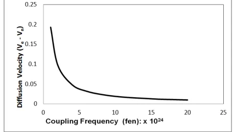
The plasma medium of the Earth’s planetary ionosphere is highly coupled due to the interactions of plasma species as they move with their respective thermal velocities [15, 33, 41]. The electrons have higher thermal velocity therefore; tend to move further away from the comparatively massive ions and in the process set up a polarization current as a result of charge imbalance which drags the ions along with the electrons. This results in ambipolar diffusion as the coupled species move through the plasma interacting with the neutral gas, and electric and magnetic fields in the terrestrial environment [3, 15]. The velocity of these coupled species as a function of collision frequency is shown in figure 1. The profile shows that the electron diffusion velocity decreases as the coupling frequency increases.

Figure 1. Variation of Diffusion Velocity with Coupling Frequency.

Figure 2. Variation of Diffusion Velocity with Electric-Magnetic Field Ratio.

The curve for the small coupling frequency indicates a much larger velocity growth rate than that for large coupling frequency as the E/B ratio increases. Further analysis shows that when the E/B ratio is much greater than one (i.e. E/B

>>

1, which implies that B ➝ 0, or that B is along E direction, or that the magnetic field component is negligible compared to the electric field); the ionized species oscillates along the direction of the electric field and thereby leading to increase in the diffusion velocity in the vertical direction. But, when the ratio is far less than one (i.e., E/B

<<

1) the magnetic field component become much larger than the electric field; therefore, the species moves along the electric field in the perpendicular direction of the magnetic field, the Lorentz forces act on them setting up a torque such that they gyrate in response to the magnetic flux. This results in a reduction of diffusion rate. The flow of plasma across magnetic field lines depends on the ratio of the coupling frequency, fkn, to the gyro-frequency, Ωk [43]. The analysis

indicates that for fkn

>

Ωk, the collision prevents the plasma

from gyrating along the magnetic field lines, instead they move in the electric field direction. But, for fkn<Ωk, the

plasma species gyrates along the magnetic field lines. The variation of coupling frequency, fkn as the electron density

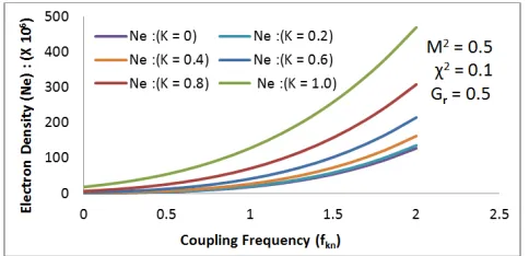
increases for different wave numbers at constant magnetic strength (M2 = 0.5) is shown in figure 3.

Figure 3. Variation of Electron Density against Coupling Frequency.

Similarly, the profiles presented in figures (4) and (5) indicate that the plasma conductivity (

δ

p) increases with electron density as well as with the height of the ionosphere. At the peak electron density which is at about 450 km up into the ionosphere, the conductivity attains maximum value and tappers off as the ionization density reduces. These findings are in agreement with those of [3, 43].

Figure 4. Variation of Plasma Conductivity with Electron Density.

Figure 5. Variation of Plasma Conductivity with Height of Ionosphere.

On the whole, the general analysis shows that when

(•9* € )9

• D(€ ,• D)≥ 0, the plasma interactive state becomes more

stable, otherwise some bit of oscillation is noticed. The stability is seen to depend among others on the magnetic field strength (E ) and thermal convection (~ ). Under this condition the signal propagation becomes less diffuse when the frequency is far greater than the plasma frequency, that is,

p >>

ω ω .

The overall analysis presented in this work aids our understanding of the physics of signal and satellite propagation in the present of ambipolar diffusion.

5. Conclusion

Ambipolar diffusion, which results from the interactions in a weakly ionized plasma, has been found to have a profound effect on the interactive state and the flow structure of ionospheric plasma. The stability condition observed in the study, aside from shedding a light on the physics and ionospheric plasma interactions, will serve as a veritable tool in mitigating factors affecting signal propagation in navigational satellites and global positioning systems.

References

[1] Carozzi, T. D. (2000); Radio Waves in the Ionosphere Propagation, generation and detection, IRF Scientific Report 272.

[3] Balan, N. (2007); Planentary Ionosphere, Kodaikanal Obseratory, Indian Institute of Astrophysics.

[4] Onwuneme, S. E. (2009); F-Layer peak electron density variations in the ionosphere, African J. Phys, 2, 45-57. [5] Abbey, T. M., Alagoa, K. D. and Onwuneme, S. E., (2011);

Propagation of MHD waves in stratified electron-plasma of the ionosphere, African J. Phys. 3, 103-119.

[6] Zolesi, B. and Cander, L. R. (2014); Ionospheric Prediction and Forecasting, Springer Geophysics, © Springer-Verlag Berlin Heidelberg.

[7] Kane, R. P. (1992); Sunspots, solar radio noise, solar EUV and Ionospheric fo2, J. Atmos. Terr. Phys., 54, 463-466.

[8] Balan, N., Bailey, G. J., Jenkins, B., Rao, P. B. and Moffett, R. J. (1994); Variations of ionospheric ionization and related solar fluxes during an intense solar cycle, J. Geophys. Res., 99(A2), 2243-2253.

[9] Balan, N., Bailey, G. J. and Moffett, R. J. (1994); Modeling studies of ionospheric variations during an intense solar cycle, J. Geophys. Res., 99(A9), 17467-17475.

[10] Leake, J. E., DeVore, C. R., Thayer, J. P., Burns, A. G., Crowley, G., Gilbert, H. R., Huba, J. D., Krall, J., Linton, M. G., Lukin, V. S., Wang, W., (2016); Chromosphere and Earth’s Ionosphere/Thermosphere, arXiv:1310.0405v4 [astro-ph.SR]. [11] Elmegreen, B. G. (1979); ApJ, 232, 729.

[12] Myers, P. C. (1985); Protostars and Planets II, ed. M. S. Matthews and D. C. Black (Tucson, AZ: Univ. Arizona Press), 81.

[13] Van Loo S., FalleS. A. E. G., Hartquist1, T. W. and Barker, A. J., (2008); The effect of ambipolar resistivity on the formation of dense cores, Astronomy and Astrophysics manuscript no. version 2.

[14] Choi Eunwoo, Jongsoo Kim and Paul J. Wiita (2009); An explicit scheme for incorporating ambipolar diffusion in a magnetohydrodynamics code, The Astrophysical Journal Supplement Series181, 413.

[15] Bai, Xue-Ning and Stone, M. James (2011); Effect of ambipolar diffusion on the non-linear evolution of Magnetorotational Instability in weakly ionized disks, Princeton University, Princeton, NJ, 08544.

[16] Mestel, L. and Spitzer, L., Jr. (1956); MNRAS, 116, 503. [17] Mouschovias, T. Ch. (1976); ApJ, 207, 141.

[18] Shu, F. H., Adams, F. C., and Lizano, S. (1987); Ara, A25, 23. [19] Committee on Solar and Space Physics, National Research

Council (2004); Plasma Physics of the Local Cosmos, The National Academies Press, Washington, D. C.

[20] Tóth, G. (1994); ApJ, 425, 171.

[21] Mac Low, M.-M., Norman, M. L., Königl, A., and Wardle, M. (1995); ApJ, 442, 726.

[22] Mac Low, M.-M. and Smith, M. D. (1997); ApJ, 491, 596. [23] Smith, M. D. and Mac Low, M.-M. (1997); AandA, 326, 801. [24] Stone, J. M. (1997); ApJ, 487, 271.

[25] Li, P. S., McKee, C. F., and Klein, R. I. (2006); ApJ, 653, 1280.

[26] Tilley, D. A. and Balsara, D. S. (2008); MNRAS, 389, 1058. [27] Padoan, P., Zweibel, E., and Nordlund, A. (2000); ApJ, 540,

332.

[28] Falle, S. A. E. G. (2003); MNRAS, 344, 1210.

[29] O'Sullivan, S. and Downes, T. P. (2006); MNRAS, 366, 1329. [30] O'Sullivan, S. and Downes, T. P. (2007); MNRAS, 376, 1648. [31] Oishi, J. S. and Mac Low, M.-M. (2006); ApJ, 638, 281. [32] Li, P. S., McKee, C. F., Klein, R. I., and Fisher, R. T. (2008);

ApJ, 684, 380.

[33] Pandey, B. P. (2016); The magnetohydrodynamic description of Earth´s ionosphere, arXiv: 1610.03735v1 [physics.plasm-ph].

[34] Cheng, P. (1964); Two-Dimensional radiating gas flow by moment method, AIAAJ 2 1662.

[35] Bestman A. R. (1983); Low Reynolds number flow in a heated tube of varying section, J. Austral. Math. Soc. Ser. B. 25, 244–260.

[36] Abbey, T. M, Bestman, A. R. and Mbeledeogu, I. U. (1992); Flow of a Two-component plasma model in a porous rotating hot sphere, Astrophys and Space Sci, 197, 67-76.

[37] Abbey, T. M. and Bestman, A. R. (1995); Slip flow in a two-component plasma model with radiative heat transfer, International Journal of Energy Research, 19: 1–6.

[38] Alagoa, K. D., Tay, G. and Abbey, T. M. (1999); Radiative and convective effects of A MHD flow through a porous medium sandwiched between two infiniteparallel plates with time dependent suction, Astrophysics and space Science, 260,455-468.

[39] Sanderson, J. J. (1974); Plasma waves in plasma physics lecture series, Edited by B. E. Keen, Institute of physics (IOP) - Publishers London.

[40] Priest, E. R. (1982); Solar magneto-hydrodynamics 1, D. Reidel Publishing Company, Holland.

[41] Steven, J. Schwartz, Christopher, J. Owen1, and David Burgess (2002); Astrophysical Plasmas, Astronomy Unit, Queen Mary, University of London, London E1 4NS, U.K. [42] Desch, S. J. (2004); Linear Analysis of the Magnetorotational

Instability including ambipolar diffusion with application to protoplanetary disks, The Astrophysical Journal, 608: 509-525.