HEAT TRANSFER OPTIMIZATION OF SHELL AND
TUBE HEAT EXCHANGER THROUGH CFD
ANALYSIS
Prof. Abhay Bendekar¹,
Prof. V. B. Sawant²
¹Asst. Professor, Mechanical Engineering ,
Shree L. R.Tiwari College of Engineerin , Thane (E), (India)
²Asst. Professor, Mechanical Engineering ,
Rajiv Gandhi Institute of Technology, Andheri (W), Mumbai, (India))
ABSTRACT
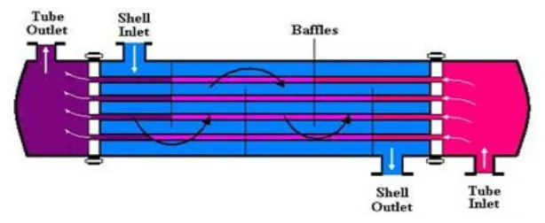
An un-baffled shell-and-tube heat exchanger design with respect to heat transfer coefficient and pressure drop
is investigated by numerically modeling. The heat exchanger contained 19 tubes inside a 5.85m long and
108mm diameter shell. The flow and temperature fields inside the shell and tubes are resolved using a
commercial CFD package considering the plane symmetry. A set of CFD simulations is performed for a single
shell and tube bundle and is compared with the experimental results. The results are found to be sensitive to
turbulence model and wall treatment method. It is found that there are regions of low Reynolds number in the
core of heat exchanger shell. Thus, k −ω SST model, with low Reynolds correction, provides better results as
compared to other models. The temperature and velocity profiles are examined in detail. It is seen that the flow
remains parallel to the tubes thus limiting the heat transfer. Approximately, 2/3rd of the shell side fluid is
bypassing the tubes and contributing little to the overall heat transfer. Significant fraction of total shell side
pressure drop is found at inlet and outlet regions. Due to the parallel flow and low mass flux in the core of heat
exchanger, the tubes are not uniformly heated. Outer tubes fluid tends to leave at a higher temperature
compared to inner tubes fluid. Higher heat flux is observed at shell’s inlet due to two reasons. Firstly due to the
cross-flow and secondly due to higher temperature difference between tubes and shell side fluid. On the basis of
these findings, current design needs modifications to improve heat transfer.
Keywords-Heat transfer, Shell-and-Tube Heat exchanger, CFD, Un-baffled.
I.
INTRODUCTION
drop. A better presentation of its efficiency is done by calculating over all heat transfer coefficient. Pressure drop and area required for a certain amount of heat transfer, provides an in- sight about the capital cost and power requirements (Running cost) of a heat exchanger. Usually, there is lots of literature and theories to design a heat exchanger according to the requirements. A good design is referred to a heat exchanger with least possible area and pressure drop to fulfill the heat transfer requirements [1].
Fig. 1 Counter-current Heat Exchanger Arrangement
A Heat Exchanger Classification
At present heat exchangers are available in many configurations. Depending upon their application, process fluids, and mode of heat transfer and flow, heat exchangers can be classified [2].
Heat exchangers can transfer heat through direct contact with the fluid or through indirect ways. They can also be classified on the basis of shell and tube passes, types of baffles, arrange- ment of tubes (Triangular, square etc.) and smooth or baffled surfaces. These are also classified through flow arrangements as fluids can be flowing in same direction (Parallel), opposite to each other (Counter flow) and normal to each other (Cross flow). The selection of a particular heat exchanger configuration depends on several factors. These factors may include the area requirements, maintenance, flow rates, and fluid phase.
B Applications of Heat exchangers
Applications of heat exchangers are a very vast topic and would require a separate thorough study to cover each aspect. Among the common applications are their use in process industry, mechanical equipment’s industry and home appliances. Heat exchangers can be found employed for heating district systems, largely being used now days. Air conditioners and refrigerators also install the heat exchangers to condense or evaporate the fluid. Moreover, these are also being used in milk processing units for the sake of pasteurization. The more detailed applications of the heat exchangers can be found in the Table 1.1 w.r.t different industries[3].
C Literature Survey
heat exchanger design [6]. These correlations are developed for baffled shell and tube heat exchangers generally.
Our study aims at studying simple un-baffled heat exchanger, which is more similar to the double pipe heat exchangers. Almost no study is found for an un-baffled shell and tube heat exchanger. Thus general correlations of heat transfer and pressure drop for straight pipes can be useful to get an idea of the design. Generally there has been lot of work done on heat transfer [7] and pressure drop [8] in heat exchangers. Pressure drop in a heat exchanger can be divided in three parts. Mainly it occurs due to fanning friction along the pipe. In addition to this it also occurs due to geometrical changes in the flow i.e. contraction and expansion at inlet and outlet of heat exchanger [9]. Handbook of hydraulic resistance pro- vides the correlations for the pressure losses in these three regions separately by introducing the pressure loss coefficients.
Compared to correlation based methods, the use of CFD in heat exchanger design is limited. CFD can be used both in the rating, and iteratively in the sizing of heat exchangers. It can be particularly useful in the initial design steps, reducing the number of tested prototypes and providing a good insight in the transport phenomena occurring in the heat exchangers [11]. To be able to run a successful full CFD simulation for a detailed heat exchanger model, large amounts of computing power and computer memory as well as long computation times are required. Without any simplification, an industrial shell and tube heat exchanger with 500 tubes and 10 baffles would require at least 150 million computational elements, to resolve the geometry [12]. It is not possible to model such geometry by using an ordinary computer. To overcome that difficulty, in the previous works, large scale shell-and-tube heat exchangers are modeled by using some simplifications. The commonly used simplifications are the porous medium model and the distributed resistance approach. Shell-and-tube heat exchangers can be modeled using distributed resistance approach [12]. By using this method, a single computational cell may have multiple tubes; therefore, shell side of the heat exchanger can be modeled by relatively coarse grid. Kao et al [13] developed a multidimensional, thermal-hydraulic model in which shell side was modeled using volumetric porosity, surface permeability and distributed resistance methods. In all of these simplified approaches, the shell side pressure drop and heat transfer rate results showed good agreement with experimental data.
With the simplified approaches, one can predict the shell side heat transfer coefficient and pressure drop successfully, however for visualization of the shell side flow and temperature fields in detail, a full CFD model of the shell side is needed. With ever increasing computational capabilities, the number of cells that can be used in a CFD model is increasing. Now it is possible to model an industrial scale shell- and-tube heat exchanger in detail with the available computers and software’s. By modeling the geometry as accurately as possible, the flow structure and the temperature distribution inside the shell can be obtained. This detailed data can be used for calculating global parameters such as heat transfer coefficient and pressure drop that can be compared with the correlation based or experimental ones[6]. Moreover, the data can also be used for visualizing the flow and temperature fields which can help to locate the weaknesses in the design such as recirculation and relaminarization zones.
functions along with k − ε models predicts the reattachment lengths more accurately, but two layer model represents the overall flow domain much better. The use of these near wall treatments is very much dependent upon the choice of turbulence model used.
II.
TURBULENCE MODELING
Turbulent flows contain a wide range of length, velocity and time scales and solving all of them makes the costs of simulations large. Therefore, several turbulence models have been developed with different degrees of resolution. All turbulence models have made approximations simplifying the Navier-Stokes equations. There are several turbulence models available in CFD software’s including the Large Eddy Simulation (LES) and Reynolds Average Navier- Stokes (RANS). There are several RANS models available depending on the characteristic of flow, e.g., Standard k − ε model, k − ε RNG model, Realizable k − ε, k − ω and RSM (Reynolds Stress Model) models.
III.
CFD ANALYSIS
Computational fluid dynamic study of the system starts with building desired geometry and mesh for modeling the domain. Generally, geometry is simplified for the CFD studies. Meshing is the discretization of the domain into small volumes where the equations are solved by the help of iterative methods. Modeling starts with defining the boundary and initial conditions for the domain and leads to modeling the entire system domain. Finally, it is followed by the analysis of the results.
A Geometry
Heat exchanger geometry is built in the ANSYS workbench design module. Geometry is simplified by considering the plane symmetry and is cut half vertically. It is a counter current heat exchanger, and the tube side is built with 11 separate inlets comprising of 8 complete tubes and3 half tubes considering the symmetry. The shell outlet length is also increased to facilitate the modeling program to avoid the reverse flow condition. In the Figure 2 (a ) and 2(b)), the original geometry along with the simplified geometry can be seen.
B Mesh
Initially a relatively coarser mesh is generated with 1.8 Million cells. This mesh contains mixed cells (Tetra and Hexahedral cells) having both triangular and quadrilateral faces at the boundaries. Care is taken to use structured cells (Hexahedral) as much as possible, for this reason the geometry is divided into several parts for using automatic methods available in the ANSYS meshing client. It is meant to reduce numerical diffusion as much as possible by structuring the mesh in a well manner, particularly near the wall region. Later on, for the mesh independent model, a fine mesh is generated with 5.65 Million cells. For this fine mesh, the edges and regions of high temperature and pressure gradients are finely meshed.
C Boundary Conditions
TABLE 1 Heat Exchanger Dimensions
IV.
RESULTS AND DISCUSSION
A Model Comparison
Different turbulence models are evaluated to investigate their application for our case. Each turbulence model along with different wall treatment methods is used with medium mesh (2.2 million cells). A comparison of overall heat transfer coefficient and pressure drop obtained from these models can be seen in the Figures 3 and 4 respectively. Knowing the temperatures from CFD results, Overall heat transfer coefficient is calculated from equations. Due to the available experimental data for comparison, only overall heat transfer coefficient is
BC Type
Shell
Tube
Inlet
Velocity-inlet
1.2 m/s
1.8 m/s
Outlet
Pressure-outlet
0
0
Wall
No slip condition
No heat flux
Coupled
Turbulence
Turbulence Intensity
3.6%
4%
Length Scale
0.005
0.001
Temperature
Inlet temperature
317K
298K
Mass flow rate
20000kg/hr
20000kg/hr
No.
Description
Unit
Value
1
Overall dimensions
mm
54x378x5850
2
Shell diameter
mm
108
3
Tube outer diameter
mm
16
4
Tube inner diameter
mm
14.6
5
Number of tubes
19
6
Shell/ Tube length
mm
5850
7
Inlet length
mm
70
calculated. Whereas, pressure drop can easily be calculated from CFD and thus, is compared with available experimental data.
Fig. 3 Overall Heat Transfer Coefficient
Fig. 4 Pressure Drop
TABLE 2 CFD and Experimental Results
B CFD Comparison with Experimental Results
On the basis of findings in previous Chapter, SST k − ω model with low Re modification is used with different mass flow rates to compare with experimental results. The results are given in the TABLE 1.
(straight tubes) is predicted with an average error between 5-9%. It can be due to small baffles in the tubes used in the experimental setup.
Overall heat transfer coefficient comparison with experiments can also be seen in the Figure6. It is also been under-predicted by this model but still better than other models with an average error of 19-20%. The good thing about these results is the constant difference from experimental results and consistency with the real systems, i.e. with higher pressure drop, higher heat transfer is achieved.
Fig. 4 Comparison of Shell Side Pressure Drop
Fig. 5 Comparison of Tube Side Pressure Drop
Fig. 6 Comparison of Overall Heat Transfer Coefficient
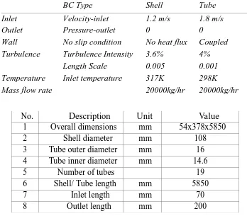
C Contour Plots
The temperature and velocity distribution along the heat exchanger can be seen through side view on the plane of symmetry. The contour plots in Figure 7 and 8 show the whole length of heatexchanger. The whole length is too much to be displayed on a single page with understandable resolution, thus it is cut into 4 parts to see it closely. The top most part is the inlet region and lowest part is the outlet.
convenience the plots are taken at 5 different positions and the details of the temperature distribution in comparison to the velocity distribution can be observed in the Table 4.1.
Fig. 7 Velocity Contour Plot at Symmetrical Plane
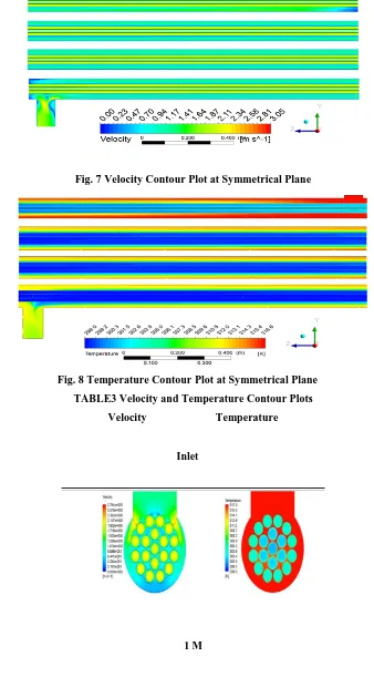
Fig. 8 Temperature Contour Plot at Symmetrical Plane TABLE3 Velocity and Temperature Contour Plots
Velocity Temperature
Inlet
3M
5M
Outlet
D Vector Plots
Fig. 9 Vector Plot of Velocity at Inlet
Fig. 10 Vector Plot of Velocity at Outlet
E Profiles
Temperature and velocity profiles are very useful to understand the heat transfer along with the flow distribution. The temperature profiles are drawn across the cross section and along the lengthof heat exchanger at different positions. Whereas, the velocity profiles are drawn only across the cross section. In order to understand the profiles, following Figures 11(a) and 11(b) must be understood first.
(a) Cross-Section (b) Length
F Velocity Profile
Fig. 12 Velocity Profiles Across the Cross-section at Different Positions in the Heat Exchanger
G Temperature Profiles
Fig. 13 Temperature Profiles Across the Cross-section of the shell at Different Positions in the Heat Exchanger
Fig15 Mass Averaged Shell and Tube side Temperatures
Fig. 16 Shell and Tube Side Temperature Profiles along the Length of Heat Exchanger
H Pressure Drop and Heat Transfer
Pressure drop along the length of heat exchanger can be seen in the Figure 18. It depicts the static pressure at inlet and outlet regions and along the length of tubes at different inlet velocities. The steeper inclination at the beginning and end of the graph shows the higher pressure drops atinlet and outlet regions. As described earlier, this happens due to cross-flow and impingement of the flow at inlet and outlet of the heat exchanger. Subsequently, heat transfer at these regions is higher as compared to the rest of heat exchanger. It can be seen in the Figure 19 that local heat transfer coefficient is very high at the inlet. This is due to several reasons, mainly being the cross flow at inlet. In addition, the temperature difference between the shell side and tube side fluid is much higher as observed in Figure16.
Fig.18 Shell Side Pressure Drop along the Length of Heat Exchanger
Fig.19: Heat Transfer Coefficient along the Length of Heat Exchanger
V.
CONCLUSION
The heat transfer and flow distribution is discussed in detail and proposed model is compared with the experimental results as well. The model predicts the heat transfer and pressure drop with an average error of 20%. Thus the model still can be improved. The assumption of plane symmetry works well for most of the length of heat exchanger except the outlet and inlet regions where the rapid mixing and change in flow direction takes place. Thus improvement is expected if complete geometry is modeled. Moreover, SST k − ω model has provided the reliable results given the y+ limitations, but this model over predicts the turbulence in regions with large normal strain (i.e. stagnation region at inlet of the shell). Thus the modeling can also be improved by using Reynolds Stress Models, but with higher computational costs. Furthermore, the enhanced wall functions are not used in this project due to convergence issues, but they can be very useful with k − ε models.
tubes. It will allow the outer shell fluid to mix with the inner shell fluid and will automatically increase the heat transfer.
REFERENCES
[1] “Aheat exchanger applications general.” Heat_exchanger/heat_exchanger_application.htm, 2011.
[2] S. Kakac and H. Liu, “Heat exchangers: Selection, rating, and thermal performance,” 1998.
[3] http://www.wcr-regasketing.com,“Heat exchanger applications.” Http://Www.wcr-regasketing.com/heat-exchanger-applications.htm, 2010.
[4] D. Kern, Process Heat Transfer. Mcgraw-Hill, 1950.
[5] R. Serth, Process Heat Transfer, Principles and Applications. Elsevier Science and Tech- nology Books.
[6] E. Ozden and I. Tari, “Shell side cfd analysis of a small shell-and-tube heat exchanger,”Energy Conversion
and Management, vol. 51, no. 5, pp. 1004 – 1014, 2010.
[7] J. J. Gay B, Mackley NV, “Shell-side heat transfer in baffled cylindrical shell and tube exchangers- an electrochemical mass transfer modelling technique,” Int J Heat Mass Trans- fer, vol. 19, pp. 995–1002, 1976.
[8] G. V. Gaddis ES, “Pressure drop on the shell side of shell-and-tube heatexchangers with segmental baffles,” ChemEng Process, vol. 36, pp.149–59, 1997.
[9] F. E. Idelchik, I.E., Handbook of hydraulic resistance. Hemisphere Publishing,New York, NY, second ed., 1986.
[10] M. J. Van Der Vyver H, Dirker J, “Validation of a cfd model of a three dimensional tube- in-tube heat exchanger.,” 2003.
[11] S. B., “Computational heat transfer in heat exchangers,” Heat Transfer Eng, pp. 24:895–7,2007.
[12] A. M. Prithiviraj M, “Shell and tube heat exchangers. Part 1: foundation and fluid mechan- ics,” Heat
Transfer, p. 33:799–816., 1998.
[13] K. T. C. S. Sha WT, Yang CI, “Multidimensional numerical modeling of heat exchangers.,”Heat Transfer, vol. 104, pp. 417–25, 1982.
[14] N. B. M. Bhutta, M.A.A Hayat, “Cfd applications in various heat exchangers design: AReview,” Applied Thermal Engineering, vol. 32, pp. 1–12, 2011.
[15] J. G. Jae-Young, K. Afshin, “Comparison of near-wall treatment methods for high reynolds number backward-facing step flow,” Int. J Computational Fluid Dynamics, vol. 19, 2005.
[16] E. Cao, Heat Transfer in Process Engineering. Mcgraw Hill, 2009.
[17] B. Andersson, R. Andersson, L. Ha˚kansson, M. Mortensen, R. Sudiyo, and B. V. Wachem,Computational
Fluid Dynamics for Chemical Engineers. Sixth ed., 2010.
[18] H. K. Versteeg and M. W., An Introduction to Computational Fluid Dynamics, The FiniteVolume Method. Pearson Education Limited, 2007.
[19] “Ansys fluent theory guide.” Http://www.ansys.com, 2010.