Building efficient fuzzy regression trees
for large scale and high dimensional problems
Javier Cózar
1*, Francesco Marcelloni
2, José A. Gámez
1and Luis de la Ossa
1Introduction
Regression trees (RTs) are light but powerful models that have been extensively used in different application domains [13, 24, 35, 37]. Their main advantage relies on their sim-plicity both in the learning and execution phases. Furthermore, RTs are highly interpret-able models, that is, they can be used to describe the relation between the inputs and the output. An RT is a tree-shaped directed graph in which each internal (non-leaf) node represents a test on an attribute and each leaf node holds an output value. Each branch, which consists of a sequence of non-leaf nodes (tests) and a leaf node (output value), represents a possible outcome for such group of tests. By following the corresponding branches from the root node to a leaf, one can find an explanation of how the output has been determined. In the literature, several different algorithms for learning RTs have been proposed [5, 20, 36].
The type of tests used in the internal nodes determines the partitioning of the input space. Given a parent node, the test acts as a splitting method for generating its child nodes. There are two main categories of RTs: binary and multi-way RTs. Binary RTs
Abstract
Regression trees (RTs) are simple, but powerful models, which have been widely used in the last decades in different scopes. Fuzzy RTs (FRTs) add fuzziness to RTs with the aim of dealing with uncertain environments. Most of the FRT learning approaches proposed in the literature aim to improve the accuracy, measured in terms of mean squared error, and often neglect to consider the computation time and/or the memory requirements. In today’s application domains, which require the management of huge amounts of data, this carelessness can strongly limit their use. In this paper, we propose a distributed FRT (DFRT) learning scheme for generating binary RTs from big datasets, that is based on the MapReduce paradigm. We have designed and implemented the scheme on the Apache Spark framework. We have used eight real-world and four synthetic datasets for evaluating its performance, in terms of mean squared error, computation time and scalability. As a baseline, we have compared the results with the distributed RT (DRT) and the Distributed Random Forest (DRF) available in the Spark MLlib library. Results show that our DFRT scales similarly to DRT and better than DRF. Regarding the performance, DFRT generalizes much better than DRT and similarly to DRF.
Keywords: Fuzzy regression trees, Big Data, Fuzzy discretizer, Apache Spark
Open Access
© The Author(s) 2018. This article is distributed under the terms of the Creative Commons Attribution 4.0 International License (http://creat iveco mmons .org/licen ses/by/4.0/), which permits unrestricted use, distribution, and reproduction in any medium, provided you give appropriate credit to the original author(s) and the source, provide a link to the Creative Commons license, and indicate if changes were made.
RESEARCH
recursively split the input space into two subspaces for each test node, so that each par-ent node is connected exactly to two child nodes. On the other hand, multi-way RTs split the input space into k partitions, where k>1 . Therefore, each parent node is connected
to a not fixed number of child nodes. The structure of a multi-way RT is usually more
compact and interpretable than the structure of a binary RT [3, 22]. On the other hand,
multi-way splits lead to more accurate RTs but, since they tend to fragment the training
data very quickly [19], they generally need larger training datasets to work effectively
[22]. Furthermore, a multi-way RT can be also represented as a binary RT [14].
One of the main drawbacks of RTs is related to the crisp bounds of the branch condi-tions: a small change in the values of the input variables may produce an important dif-ference in the prediction. To overcome this problem, RTs have been extended with the
use of fuzzy set theory, originating fuzzy regression trees (FRTs) [31, 39]. FRTs employ
fuzzy conditions in their internal nodes. Therefore, an input can enable several branches in a test node, and reach different leaves, with different confidence levels. The output value of the FRT is obtained by appropriately combining the values associated with these multiple leaf nodes. FRTs are, in general, more complex both in learning and execution phases than RTs.
Fuzzy regression tree learning algorithms usually apply an initial discretization step aimed at generating fuzzy partitions on the continuous input variables, typically guided by some purposely-defined index [43, 47]. Since this step has a direct impact on the per-formance of the learning algorithm, several studies evaluate how the accuracy and com-plexity of the generated models depend on the discretization [15, 23, 50].
Most of FRT learning algorithms proposed in the literature focus on the accuracy but
do not consider the computation complexity and space requirements [33, 39]. Typically,
these algorithms have been tested and assessed on small datasets, and are not generally suitable for managing huge amounts of data. In fact, one solution often adopted to work in real contexts with these algorithms, is to reduce the dataset by applying downsam-pling techniques. However, these techniques may cut off some useful knowledge, mak-ing FRT learnmak-ing approaches purposely designed for managmak-ing the overall dataset more desirable and effective. Thus, we aim to learn FRTs from the overall dataset, indepen-dently of its size. In other words, we desire to cope explicitly with Big Data.
As described in [42], Big data refers to the storage and analysis of large and/or
com-plex data sets using a series of specific techniques. These techniques combine new
para-digms (software) together with specific hardware architectures. A recent work [38] of
one of the co-authors has proposed a novel fuzzy decision tree algorithm to address Big Data classification problems. First, the domain of the continuous input features is
discre-tized by adopting a distributed approach based on the fuzzy entropy concept [50]. Then,
the fuzzy decision tree is learned by applying a distributed learning algorithm based on the fuzzy information gain concept. Both phases have been implemented by using the MapReduce paradigm in the Apache Spark framework.
In this paper, we adapt the algorithm proposed in [38] to deal with Big Data regression
eight real-world datasets [2] and four synthetic datasets [40]. The results are discussed in terms of mean squared error, computation time and scalability, and compared with the ones achieved by the distributed regression tree and the Distributed Random Forest
[4], both included in the MLlib Apache Spark library [30]. To the best of our
knowl-edge, the proposed algorithm is the first distributed FRT learning scheme proposed in the literature.
The paper is organized as follows. “Background” section introduces some preliminary
concepts about RTs and FRTs. Afterwards, in “MapReduce and spark” section, we briefly
discuss MapReduce and Apache Spark. “Fuzzy regression tree for Big Data” section
describes our proposed FRT learning algorithm and presents its distributed
implemen-tation. Then, in “Results and discussion” section, we present the experimental results.
Finally, in “Conclusions” section, we draw our conclusions.
Background
In classification problems, a class cm from a predefined set C= {c1,. . .,cM} of M classes is assigned to an unlabeled instance. A classification problem is defined by a set of input variables X= {X1,. . .,XF} and the output Y. In case of numerical variables, Xf is defined on a universe Uf ⊂R . In case of categorical variables, Xf is defined on a set Lf = {Lf,1,. . .,Lf,Tf} of categorical values.
Decision trees (DTs) have been widely used in instance classification problems [11, 16,
52]. A DT is a tree-shaped directed graph in which each internal (non-leaf) node
repre-sents a test on an attribute. Each path from the root to a leaf corresponds to a sequence of tests, which aims to isolate a subspace of the input space. The objective of the test is to partition the training set into subsets as pure as possible, that is, subsets composed by instances belonging to the same class. In the case of numerical variables, tests are defined by intervals in the definition domain; in the case of categorical variables, they correspond to subsets of the possible categorical values. Formally, tests are in the form of Xf >xf,s and Xf ≤xf,s for numerical input variables, and Xf ⊆Lf,s for categori-cal input variables, where xf,s and Lf,s are a numeric threshold and a set of categorical values for the test s, respectively. Each leaf node is characterized by a class cm ∈C: the instances, which satisfy the overall sequence of tests from the root to the leaf, are classi-fied as belonging to cm.
Decision trees can also be used in regression problems, named regression trees (RTs). The objective is to predict a real value rather than a class label. Thus, leaf nodes are characterized by a regression model defined over the input variables. For instance M5 [36] generates first-order polynomials using the overall set of input variables. CART [5], which is one of the most known algorithms for generating regression trees, uses zero-order polynomials i.e. a numerical constant, leading to simpler and usually more robust models. Indeed, the use of high order polynomials tends to overfit.
In this work, we focus on zero-order polynomial fuzzy regression trees (FRTs) [18].
Each real input variable is partitioned by using fuzzy sets. The tests in the internal nodes use these fuzzy sets in the form of Xf is Bf,t, where Bf,t is a fuzzy set defined over the
variable Xf. The membership degree of a value xi,f with respect to the fuzzy set Bf,t is
represented as µBf,t(xi,f). Similarly, the membership degree of an instance xi with respect to the fuzzy sets B1,t1,. . .,BF,tF is represented as T-Norm
B1,t1(xi),. . .,BF,tF(xi)
is a conjunction of the individual membership degrees.1 Since fuzzy sets generally over-lap, an input instance may activate more than one leaf node. The value assigned to each leaf node is computed as a weighted average of the output values for all the training set instances that activate such leaf node, using the activation degrees as instance weights.
There are different approaches for generating the fuzzy partitions of the input
vari-ables automatically from data [23, 27, 50]. Most of them use two steps: discretization
and fuzzy partition generation. The first step consists of discretizing the domain of each input variable into a finite set of disjoint bins. To this aim, different strategies have
been proposed in the literature [17]: splitting vs. merging, supervised vs. unsupervised,
dynamic vs. static, and global vs. local. Once the bins have been generated, in the sec-ond step the membership functions of the fuzzy partition are derived from these bins by employing different methods: the use of the bin bounds to define the fuzzy sets sequen-tially ordered [34], based on histograms [29], probabilities [12], fuzzy nearest neighbors [21], neural networks [29], entropy [6], particle swarm optimization [32] or clustering
based methods [29]. In this paper, we adopt an approach that generates triangular fuzzy
partitions directly by using a single step.
Algorithm 1 shows the scheme of a generic FRT learning process, where TR= {(x1,y1),. . .,(xN,yN)} is the training set, X is the set of input variables, SplitMet is the splitting method, StopMet is the stopping method, and FRT is the output (learnt model).
The algorithm first creates the root node. Then, it builds the FRT model with the Tree-Growing recursive function. This function first checks if the node is a leaf by means of the
StopMet function. If not, it calls the function SelectBestFeatureSplits, which selects the best input variable to partition the input space. There are several metrics that can be used to perform the variable selection. However, the most popular one in zero-order FRTs is the variance [7, 10]. Finally, for each splitz in splits the TreeGrowing function creates a child node and recursively calls itself using the subset of instances, which satisfy the test for such child node.
After learning the tree structure, each leaf node ni in the set of leaf nodes, LN, estimates a regression model from the instances in the training set, which activate such leaf node, i.e.,
which satisfy the sequence of tests from the root to such leaf node. Let Sni be the set of
instances that activate the leaf node ni . RMni is the weighted average of the instances
(xl,yl)∈Sni by using their activation degree µnl i(
xl) as weight:
During the inference, the prediction is computed as follows. Let Nl =nl1,. . .,nMl
be the set of leaf nodes activated by the input instance xl with an activation degree µnl
i( xl) .
The output of the FRT is obtained as:
MapReduce and Spark
MapReduce (MR) is a programming paradigm proposed in 2004 [9] for distributing
the computation of parallel data-oriented tasks across a cluster of machines. At the beginning, it was developed as a solution to improve the performance of the Google Search Engine. Currently, its usage has been extended to process large amounts of data in multiple different areas [25].
MapReduce presents an abstraction layer to the developers: It divides the problem into smaller tasks, called Map and Reduce, and executes those tasks in parallel taking care of communication, network bandwidth, disk usage and possible failures. In this way, the developers are able to implement parallel algorithms by simply defining the Map and Reduce functions, avoiding problems related to the underlying architecture and hardware configuration. In order to execute these tasks, MR follows a master-slave scheme. First, the data is automatically divided into a set of independent blocks,
called chunks, which can be processed in parallel by different machines [26]. Then, the
master computing node configures multiple tasks, each one fed with a chunk of data, and executes them in parallel in slave computing nodes.
The data managed by the MR workflow are represented by key,value pairs.
Ini-tially, an arbitrary key is assigned to each input. Then, in the Map phase, each task processes the data by applying the defined map function, which generates a list of
intermediate key,value pairs (one per map task). Then, the system collects these
pairs, sort them according to their keys, and feed reduce tasks with the pairs shar-ing the same key. Finally, in the Reduce phase, the defined reduce function is used to
RMni =
(xl,yl)∈Sniyl·µnli(xl)
ni∈LN
(xl,yl)∈Sniµnli(xl)
(1) FRT(xl)=
ni∈NlRMni·µni(xl)
combine the list of values (which share the same key) to produce a new key,value
pair. The result of the MapReduce process is a list of key, value pairs generated by all
the executed Reduce tasks.
The most extended implementation of this paradigm is Apache Hadoop [45], where
the open-source community worked together with many private companies to pro-vide a general framework for Big Data processing. The key parts of Apache Hadoop are the MapReduce implementation and the Hadoop Distributed FileSystem (HDFS), which allows working efficiently with large amount of data following the previously described processing.
The most important drawback of Apache Hadoop is that the output is written in the hard driven storage. This decreases the performance for iterative (or stream-based)
workflows. Apache Spark [49] is a framework, which overcomes this problem by
stor-ing the data structures in the main memory (significantly faster) until the whole pro-cess finishes (the propro-cess can be a sequence of MapReduce tasks). In practice, the main difference with respect to Apache Hadoop is the resilient distributed dataset (RDD), which relax the MapReduce workflow and allows the developer to define and use additional operations over the data.
Spark has been implemented using the Scala programming language, but there are alternative languages, which can be used for developers, like Python and R. The exist-ence of such interfaces eases its usage and has made Apache Spark one of the most popular frameworks for Big Data processing, in particular within the Data Science
community. As a consequence, MLlib [48] has been developed as part of the Apache
Spark project. MLlib is a library for Apache Spark, which implements the most popu-lar machine learning algorithms following the MapReduce paradigm.
Fuzzy regression tree for Big Data
In this section, we present our FRT learning approach for big data regression problems. We have adapted the distributed fuzzy decision tree learning approach, proposed by one of the authors in [38] for handling Big Data classification problems, to deal with regression problems. The learning approach consists of two steps: the first one creates fuzzy partitions on the domains of the input variables, and the second one induces a binary FRT from data using the fuzzy partitions generated in the first step. With respect to the original approach, we have employed different measures for both evaluating the partitions in fuzzy partition-ing and for determinpartition-ing the optimal variable to be used in a decision node in the FRT learn-ing phases. Consequently, we have had to introduce different stopplearn-ing conditions. Further, we have employed some specific adjustments for speeding-up the FRT generation.
In the following, we first describe both steps and then we explain how these steps have been designed to be implemented under the MapReduce paradigm.
Fuzzy partitioning
Partitioning of continuous variables is a crucial aspect in the generation of both FDTs and
FRTs, and therefore should be performed carefully. The work in [50] evaluates several
In regression, one of the most used indexes is fuzzy variance [8]. Thus, we have adapted the recursive supervised fuzzy partitioning method proposed in [38] for classification prob-lems, by using fuzzy variance as metric. The adapted version, denoted as partitioning based on fuzzy variance (PFV), is a recursive supervised method, which generates candidate fuzzy partitions, and evaluates these partitions employing fuzzy variance rather than the fuzzy entropy as used in the classification-oriented method.
Let TRf = [(x1,f,y1),. . .,(xN,f,yN)] be the projection of the training set TR along the input variable Xf. Let us assume that the values xi,f are sorted in increasing order. Let If be
an interval defined on the universe of Xf. Let lf and uf be the lower and upper bounds of If.
Let Sf be the set of values (xi,f,yi)∈TRf contained in If. Let PIf = {Bf,1,. . .,Bf,KPI f
} be a
fuzzy partition defined on If, where KPIf is the number of fuzzy sets in PIf. Let
Sf,1,. . .,Sf,KPI
f be the subsets of points in Sf, contained in the support of Bf,1,
. . .,Bf,KPI
f, respectively.
The fuzzy mean FM(PIf) of a fuzzy partition PIf is defined as the mean of the output values yi , corresponding to the instances whose value xi,f ∈Sf , weighted by the member-ship degrees of xi,f to any Bf,j∈PIf:
The fuzzy variance FVar(PIf)
of a fuzzy partition PIf is defined as:
At the beginning of the execution of PFV, If coincides with the universe of Xf and
Sf =TRf. First of all, PFV sorts the values of TRf in ascending order. Afterward, for each
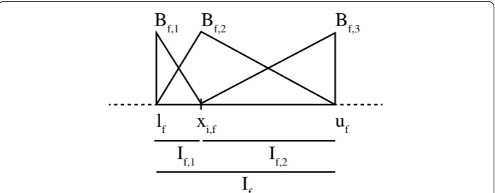
value xi,f between lf and uf (at the beginning of the partitioning procedure, i=1,. . .,N ), PFV defines a strong fuzzy partition PIf(xi,f) on If by using three triangular fuzzy sets,
namely Bf,1,Bf,2 and Bf,3, as shown in Fig. 1. The cores of Bf,1,Bf,2 and Bf,3 coincide with
lf,xi,f and uf, respectively. PFV computes FVar(PIf(xi,f)) for each fuzzy partition PIf(xi,f) induced by each xi,f and selects the optimal value x0i,f, which minimizes FVar(PIf(xi,f)).
This value identifies the fuzzy partition PI0f(x0i,f)= {B0f,1,B0f,2,B0f,3}. Let Sf0,1,Sf0,2 and Sf0,3 be the subsets of points in Sf, contained in the support of the three fuzzy sets, respec-tively. Then, PFV applies recursively the procedure for determining the optimal strong fuzzy partition to the intervals If =If0,1= [lf,x0i,f] and If =If0,2=(x0i,f,uf] identified by x0i,f, by considering Sf =Sf0,1 and Sf =S0f,3, respectively, until the following stopping con-ditions are met:
(2) FM(PIf)=
KPIf
j=1
(xi,f,yi)∈Sf,jyi·µBf,i(xj,f) KPIf
j=1
(xj,f,yi)∈Sf,jµBf,j(xi,f)
(3)
FVar(PIf)=
KPIf
j=1
(xi,f,yi)∈Sf,j(yi− FM(PIf))
2·µ2 Bf,j(xi,f)
KPIf
j=1
(xi,f,yi)∈Sf,jµ
• the cardinality |Sf| of Sf is lower than a fixed threshold disc
• the partition fuzzy gain ( PFGain(PIf) ) is lower than a fixed threshold ǫdisc
PFGain(PIf) measures the improvement in terms of fuzzy variance of the involved inter-vals. It is defined as follows:
where w(PIf,s), with s=1, 2, is defined as:
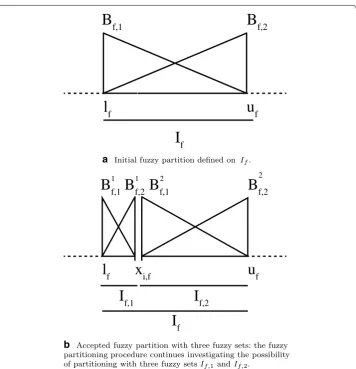
If no initial partition exists on If (this occurs when If coincides with the universe of
Xf and Sf =TRf ), we assume two fuzzy sets Bf,1 and Bf,2 defined on If, as shown in
Fig. 2a. Once the fuzzy partition with three fuzzy sets is accepted, the procedure
gen-erates a partition with three fuzzy sets from intervals If,1 and If,2 as shown in Fig. 2b. The partitioning of both If,1 and If,2 may generate three fuzzy sets in both [lf,xi,f] and
(xi,f,uf]. Actually, the two fuzzy sets, which have the core in xi,f are fused generating a unique fuzzy set. This fusion can be applied at each level of the recursion. The final result is a strong triangular fuzzy partition Pf = {Af,1,. . .,Af,Tf} on Uf, where Af,j is the j-th fuzzy set defined on Uf.
FRT learning
Once fuzzy partitions have been defined, the pseudo-code described in Fig. 1 is
employed to build the FRT. In the SelectBestFeatureSplits function, we use the expres-sion PFGain(PIf), defined in Eq. 4, to determine the best binary split. To calculate the
split with the maximum PFGain(PIf), we evaluate all possible candidates, by grouping
together adjacent fuzzy sets into two disjoint groups Z1 and Z2 . The two subsets G1 and
G2 of instances contain the points that belong to the support of the fuzzy sets contained
(4)
PFGain(PIf)=FVar(PIf)−FVar(PIf,1)·w(PIf,1)
−FVar(PIf,2)·w(PIf,2)
(5)
w(PIf,s)= KPIf,s
g=1
(xi,f,yi)∈Sf,sµ
2 Bf,g(xi,f)
KPIf
j=1
(xi,f,yi)∈Sf µ2B
f,j(xi,f)
l
fx
i,fu
fI
f,1I
f,2B
f,1B
f,2B
f,3I
fin Z1 and Z2 , respectively. A fuzzy partition with Tf fuzzy sets generates Tf −1 candi-dates. Starting with Z1= {Af,1} and Z2= {Af,2, ...,Af,Tf} , we compute the fuzzy gain by applying Eq. 4, with Pf = {Z1,Z2} and cardinality |G1| =iN=11TN(µAf,1(xf,i),µG(xi)) and |G2| =N2
i=1TN(µAf,2(xf,i)+ · · · +µAf,Tf(xf,i),µG(xi)) , where N1 and N2 are the
numbers of instances in the support of the fuzzy sets in Z1 and Z2 , respectively, and
µG(xi) is the membership degree of instance xi to the parent node. Iteratively, the algo-rithm investigates all candidates by moving the first fuzzy set in Z2 to Z1 and computing the corresponding PFGain(PIf) , until Z2= {Af,Tf} . The pair ( Z1,Z2 ), which obtains the
highest PFGain(PIf) , is used to create the two child nodes. The two nodes contain,
respectively, the examples that belong to the support of the fuzzy sets in Z1 and Z2. In case of categorical variables the computation cost can become very prohibitive:
a categorical variable with L values generates 2L−1−1 possible combinations. We
have adopted the same approach used in [38]: we reduce the possible combinations
by sorting the categorical values according to an arbitrary order (by appearance in the dataset). Afterward, we use each categorical value xj,f as splitting point: the first
l
fu
fB
f,1B
f,2I
fa Initial fuzzy partition defined on If.
l
fx
i,fu
fI
f,1I
f,2B
f,1B
f,2B
f,2I
fB
f,11 1 2 2
b Accepted fuzzy partition with three fuzzy sets: the fuzzy partitioning procedure continues investigating the possibility of partitioning with three fuzzy setsIf,1andIf,2.
subset is composed of all the values xi,f such that i≤j, leaving the rest for the second
subset. Therefore, the number of possible partitions is reduced to L−1.
The process terminates when one of the following conditions is met (StopMet procedure):
• The number of instances that reach the node is smaller than a fixed threshold
learn.
• The PFGain(PIf) is lower than a threshold ǫlearn.
• The tree has reached a maximum fixed depth β.
The output of the model is computed as in Eq. 1. As we mentioned above, in the case
of binary FRTs, an input variable can be considered more than once in the same path from the root to a leaf node, as the partitioning is done in a recursive way where an
interval If can be split into subintervals at different levels. The use of the T-Norm
tends to penalize the matching degree of the instance for those input variables that are repeatedly selected along a same path (from the root to a leaf node). To reduce this effect, we use a strategy that remembers each fuzzy set used in the path, and its membership degree is computed and used only the first time it appears; for the subse-quent times the membership degree used is 1.
Distributed approach
We have adapted the distributed implementation proposed in [38] for learning
dis-tributed fuzzy decision trees, based on the Map-Reduce paradigm and implemented in Apache Spark. Let V be the number of chunks used for splitting the training set and Q the number of computing units (CUs). Each chunk feds only one Map task, while one CU can process several tasks, both Map and Reduce. Obviously, only Q tasks can be executed in parallel.
The distributed approach follows the same procedure described in the previous sec-tions: first it generates the fuzzy partition of each input variable and then builds the distributed FRT, denoted as DFRT in the following.
With respect to the fuzzy partitioning, we use an approximation of the PFV
approach described in “Fuzzy partitioning” section. Indeed, in case of big data, the
number of possible candidate splitting points, corresponding to the different values xi,f in the training set for each input variable Xf , might lead to intractable computa-tion times. To reduce this problem, we limit the number of possible candidate split-ting points by adopsplit-ting an equi-frequency discretization of the domains of each input variable. In particular, as already used in [38], for each input variable Xf , we sort the values xi,f in the training set and partition the domain of Xf into a fixed number L of equi-frequency bins. Then, we aggregate the lists of the bin boundaries generated for each chunk and, for each pair of consecutive bin boundaries, we generate a new bin and compute the required statistics for this bin to be used for computing the fuzzy
variance at each iteration of PFV. PFV applies the same process described in “Fuzzy
partitioning” section, using the central values of such bins as candidate splitting
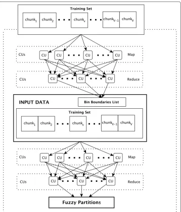
In the first phase, distributed bin generation, the Map-Reduce implementation of PFV
scans the training set to generate at most V·L bin boundaries. Each Map task loads a
chunk v of data and, for each continuous input variable Xf , sorts its values and computes L equi-frequency bin boundaries, including the left and and right extremes of the Xf domain in the chunk. Let BBv,f = {bv,f(1),. . .,bLv,f} be the sorted list of bin boundaries. The output of the Map task is a key-value pair �key=f,value=BBv,f� , where f is the index of the input variable Xf and BBv,f is the sorted list of bin boundaries. Afterwards, each
Reduce task is fed by V lists of bin boundaries for the same input variable Xf , and
out-puts a key-value pair �key=f,value=BBf� , where BBf is the sorted list of the bin boundaries for that variable Xf (obtained by joining all the bin boundaries of each BBv,f ). If the number of bins is equal to the number of values in the interval (one value per bin), it is equivalent to PFV. On the other side, the lower the value of L is, the coarser the
approximation in determining the fuzzy partition is. We choose L equal to the percent-age γdisc of the chunk size.
In the second phase, distributed fuzzy sets generation, we generate the fuzzy parti-tions for each continuous input variable. Each Map task is fed by the bin boundaries list. Let xi,f ∈S(ft,v) be the instances in the chunk v that are contained in the bin b(t)f . Then, for each input variable Xf and for each bin b(t)f in BBf, the Map task computes three statis-tics Ωt,v,f = {Ω1t,v,f,Ω2t,v,f,Ω3t,v,f}, where
• Ω1t,v,f is the sum of the outputs yi corresponding to xi,f ∈Sf(t,v);
• Ω2t,v,f is the sum of the squared outputs yi2 corresponding to xi,f ∈Sf(t,v); • Ω3t,v,f is the number of instances xi,f ∈Sf(t,v).
The output of the Map phase is a list of pairs �key=f,value=Ωt,v,f� . Each Reduce
task is fed by a list of V statistics Ωt,v,f for the input variable Xf . In a first phase, the Reduce task performs an element-wise addition for all the three statistics, obtaining Ωv,f . Finally, it applies the PFV described in “Fuzzy partitioning” section. Let b(ft) be
the central point of each bin b(t)f . In order to compute efficiently the PFGain(PIf ) given a splitting point b(t)f , we first compute the following values Gf(1,j) , G(2)f,j , G(3)f,j and Gf(4,j) by iterating over the bins instead of over the instances, with f =1. . .F and j=1,. . .,Tf:
Using Gf(1,j),Gf(2),j,Gf(3),j and G(f4,j) , FM(PIf) can be easily computed as:
(6)
Gf(1,j)=
b(ft)∈BBf
µAf,j(b
(t)
f )·Ω t,f
3
(7)
Gf(2,j)=
b(ft)∈BBf
µ2Af ,j(b
(t)
f )·Ω t,f 3
(8)
Gf(3,j)=
b(ft)∈BBf
µAf,j(b
(t)
f )·Ω t,f 1
(9)
Gf(4,j)=
b(ft)∈BBf
µ2Af
,j(b
(t)
f )·Ω t,f
2
(10)
FM(PIf)= KPIf
j=1 G
(3) f,j
KPI
f j=1 G
FVar(PIf) can be obtained as:
Finally, PFGain(PIf) is computed with Eq. 4. The output of PFV is a fuzzy partition for each input variable. These fuzzy partitions are input to the DFRT learning process.
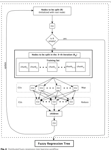
In DFRT learning, the best split for each node is computed in parallel across the
CUs. Figure 4 describes the workflow of the DFRT learning. The DFRT learning is an
iterative process, which executes a complete Map-Reduce step at each iteration. Let H be the number of iterations performed by the algorithm and h be the index of the h-th iteration. Let R be the list of nodes to be split, initialized with only one element consisting of the root of the tree. The algorithm iteratively determines the group Rh of |R| nodes from R. Finally, it performs a Map-Reduce step for distributing the growing pro-cess of the tree.
Each Map task, using the corresponding chunk v of data, computes, for each node NTy∈Rh , a vector Dv,y of size |D| = ∀f∈FTf elements. In particular,
each element j of Dv,y corresponds to the fuzzy set Af,j and its value is equal to
Dv,y[j] = Sf,j
i=1 TN(µAf,j(xf,i)·µNTy(xi)) , where µNTy(xi) is the membership degree of
instance xi to the parent node (for the root of the decision tree, the membership value
is equal to 1) and the operator TN is a T-norm. The output of these Map tasks are key-value pairs �key=y,value=Dv,y� (where y is the index of the node NTy ). Afterward, each Reduce task receives a list of vectors Dv,y and creates a vector Dy by performing an
element-wise addition of all V vectors. Thus, Dy stores the cardinality of each input
vari-able from the root to NTy along the overall training set. Then, the Reduce task generates
two child nodes and tests the stopping conditions described in “FRT learning” section
for both of them. The children generated from each NTy are used to update the tree and
R: if a child node is not labeled as leaf, then it is inserted into the list R and employed at the next iterations. The algorithm repeats all the steps until R is empty.
In order to compute the PFGain(PIf ) efficiently (used to test the second stopping crite-ria), we first compute the values Gf(1,j) , G(f,2j) , Gf(3),j and G(4)f,j (Eqs. 6–9 respectively), similar to the distributed PFV algorithm. Further, Ωl,f is already available because it was computed by the distributed PFV algorithm and µBf,j(b
(t)
f ) is obtained efficiently by computing the
T-Norm using the membership degrees stored in Dy.
Results and discussion
In order to test the behavior of the proposed DFRT, we have performed a set of experi-ments that evaluate the performance in terms of MSE, complexity and scalability related to the size of the datasets and the number of used CUs. MSE is computed as:
(11)
FVar(PIf)=
KPIf j=1
(b(ft),y(t))∈Sf,j
(y(t)−FM(PIf))2·µ2Bf,j(b(t)f )
KPIf j=1
(b(ft),y(t))∈Sf,jµ 2 Bf,j(b
(t) f )
=
KPIf j=1 G
(4) f,j +G
(1)
f,j ·FM(PIf)2−2·G (3)
f,j ·FM(PIf)
KPIf j=1 G
where DS stands for each dataset.
Complexity is calculated as the number of nodes of the tree. Scalability is presented by plotting the average execution times versus the number of CUs.
(12)
MSE =
|DS|
i=1(yi− DFRT(xi))2
|DS|
We have used 8 real world datasets [2].2 These datasets come from the same real-world problem, the Protein Structure Prediction (PSP), which aims to predict the 3D structure of a protein (output variable) based on amino-acid structural continuous
variables (inputs). As described in [1], a protein structure (PS) is the three-dimensional
arrangement of atoms in a protein molecule. These structures arise because particular sequences of amino-acids in polypeptide chains fold to generate, from linear chains, compact domains with specific 3D structures. The folded domains can serve as modules for building up large assemblies such as virus particles or muscle fibers, or they can pro-vide specific catalytic or binding sites, as found in enzymes or proteins that carry oxy-gen or regulate the function of DNA. PSP predicts the three-dimensional structures of a protein by using its first structure, its amino-acid sequence, to predict its folding and its secondary, tertiary and quaternary structure [44, 51]. This makes PSP an essential tool in proteomics since the molecular function of a protein depends on its threedimensional structure, which is often unknown.
The difference among these datasets relies on the number of input variables, varying from 100 (Window2) to 380 (Window9) by steps of 40 input variables. The number of instances is 257560 for all the datasets. To validate the results we have used a ten fold cross-validation (10-CV), being 234638 instances for training and 22922 for test at each iteration.
To the best of our knowledge few real-world big datasets exist for regression problems. Thus, with the aim of enriching the experimental evaluation and extracting more robust
conclusions, we have generated 4 synthetic datasets, following the procedure used in [40]:
two of them ( f1 and f19 , described in Eqs. 13 and 14) are characterized by 1000 input vari-ables and 105 instances, and the remaining two ( f2 and f4 , described in Eqs. 15 and 16) by
100 input variables and 106 instances. The generation process consists of generating
ran-dom instances, where each input variable has a predefined ran-domain, and applying a function over the selected input variables to produce the output value. Let x= {x1,x2,. . .,xF} be a
random input instance in a predefined domain, P a random permutation of {1, 2, …, F} and
M an orthogonal matrix of dimension m×m , where m has been fixed to 50. The
defini-tions of f1 , f19 , f2 and f4 are, respetively:
(13)
f1(x)=
F
i=1
(106)Fi−−11 ·x2
i
(14) f19(x)=
F �
i=1
i �
j=1
xi
2
(15)
f2(x)=
F
i=1
x2i −10 cos(2πxi)+10
To give a glimpse of the complexity of the problems, we have computed three metrics
proposed in [28] for evaluating the correlation between input variables and output. In
particular, we have adopted Maximum and Average Feature Correlation to the Output, and Collective Feature Efficiency, denoted as C1 , C2 and C4 , respectively, in the
origi-nal paper. C1 and C2 measure the maximum and average Spearman correlation values
between the input variables and the output (see Eqs. 17 and 18). C4 measures the
per-centage of instances which are difficult to predict (large residual values) with respect to a linear regressor (see Eq. 19).
where (xj,y) is the projection of the dataset DS along the input variable Xj , ρ(xj,y) is the Spearman correlation between the input variable Xj and the output, and sl is the number of instances which have been iteratively marked as linearly classifiable (residual obtained by a linear classifier between the feature Xj and Y smaller than 0.01), being Xj the most correlated feature with respect to Y that has not been yet selected.
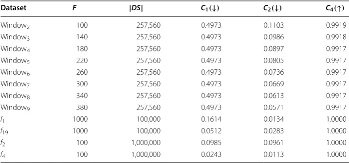
The properties for each dataset (number F of input variables, number |DS| of
instances, and metrics C1 , C2 and C4 ) are shown in Table 1. The symbols ↑ and ↓
denote that, respectively, high (direct relation) and low (indirect relation) values of the metrics correspond to high complexity. The values highlight that the problems (16) f4(x)=f1({xP1,. . .,xPm} ×M)·10
6
+f1({xPm+1,. . .,xPF)}
(17) C1= max
j=1,...,F|ρ(xj,y)|
(18)
C2=
F
j=1
|ρ(xj,y)|
F
(19) C4=1−
l sl
|DS|
Table 1 Properties of the real-world and synthetic datasets
Dataset F |DS| C1(↓) C2(↓) C4(↑)
Window2 100 257,560 0.4973 0.1103 0.9919
Window3 140 257,560 0.4973 0.0986 0.9918
Window4 180 257,560 0.4973 0.0897 0.9917
Window5 220 257,560 0.4973 0.0805 0.9917
Window6 260 257,560 0.4973 0.0736 0.9917
Window7 300 257,560 0.4973 0.0669 0.9917
Window8 340 257,560 0.4973 0.0613 0.9917
Window9 380 257,560 0.4973 0.0571 0.9917
f1 1000 100,000 0.1614 0.0134 1.0000
f19 1000 100,000 0.0512 0.0283 1.0000
f2 100 1,000,000 0.0985 0.0961 1.0000
are particularly difficult since there does not exist a high correlation between input
variables and output. In particular, the values of C4 point out that the output is very
difficult to predict by using a linear regressor. In fact, we made some additional exper-imentation using the distributed linear least squares approach implemented in the Apache Spark MLlib. The results achieved by this algorithm were very poor and thus, for the sake of brevity, we do not present them in this work.
The experiments have been executed on a cluster of computers with one master and six slave nodes equipped with dual Intel Xeon E5-2609v3 1.90 GHz hexacore proces-sors and 64GB of RAM per node. Each worker node is running the HDFS file system on 4x1TB disks and is managed by the 1.5.2 version of the Apache Spark standalone distribution.
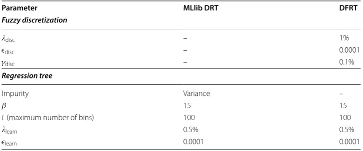
In order to validate the results of our DFRT, we have first compared them to the ones obtained by the distributed regression tree (DRT) of the MLlib Apache Spark’s implementation (from version 1.5.2). The parameters used for the execution of DRT
and DFRT are shown in Table 2. The comparison is performed in terms of MSE,
exe-cution time and scalability. Then, we have compared the results of our DFRT with the ones achieved by the Distributed Random Forests (DRFs) of the MLlib Apache Spark’s
implementation. Random Forest [4] is an ensemble of regression trees. The effect of
using an ensemble is that, asymptotically, the bias of the model is similar to the one obtained by one single tree, while the variance is significantly reduced. As this is one of the key points in fuzzy regression trees, we have compared our DFRT to DRF in
terms of variance, in addition to MSE. In “Comparison with Distributed Random
For-est” section, we present this comparison and draw some conclusions.
Comparison with DRT
We will analyze the results for the real and the synthetic datasets separately (first the
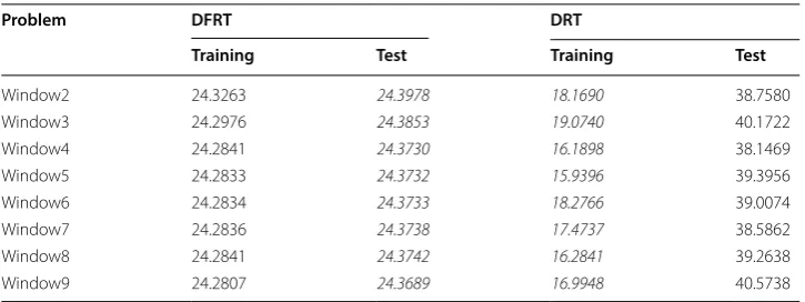
real-world problems). Tables 3 and 5 show the average training and test MSEs obtained
by our DFRT and the MLlib DRT.
Table 2 Parameters for the MLlib DRT and the DFRT
Parameter MLlib DRT DFRT
Fuzzy discretization
disc – 1%
ǫdisc – 0.0001
γdisc – 0.1%
Regression tree
Impurity Variance –
β 15 15
L (maximum number of bins) 100 100
learn 0.5% 0.5%
As we can observe in Table 3, DRT suffers from overfitting. Indeed, the training MSE is much lower than the test MSE. Further, the test MSE obtained by DRT is much higher than the one achieved by DFRT. On the other hand, the training and test MSEs obtained by DFRT are similar, thus showing that DFRT is not prone to overfitting.
Regarding the complexity, Table 4 shows the average number of nodes (inner and
leaves) and the average number of leaves. We can observe that the complexity of the models is very similar for the same algorithm for all the real-world datasets (we just observe a slight increase on the numbers of nodes and leaves in the case of DRT). From Table 1 we can observe that the real-world datasets have the same value of the C1 metric
and the C2 metric decreases with the increase of the number of inputs (from Window2 to
Window9 ). This means that the most correlated input variables belong to the shared 100
input variables (variables from Window2 ). For this reason, the results do not improve
notably by including the rest of the input variables, and therefore are very similar for these datasets. Comparing the algorithms, DRT is much more complex than DFRT in terms of numbers of both nodes and leaves (approximately a difference of one order of magnitude).
Table 3 Average MSEs obtained by DFRT and DRT on the training and test sets for the real-world problems
The best results for each dataset have been emphasized in italic font
Problem DFRT DRT
Training Test Training Test
Window2 24.3263 24.3978 18.1690 38.7580
Window3 24.2976 24.3853 19.0740 40.1722
Window4 24.2841 24.3730 16.1898 38.1469
Window5 24.2833 24.3732 15.9396 39.3956
Window6 24.2834 24.3733 18.2766 39.0074
Window7 24.2836 24.3738 17.4737 38.5862
Window8 24.2841 24.3742 16.2841 39.2638
Window9 24.2807 24.3689 16.9948 40.5738
Table 4 Average complexity of the models obtained by DFRT and DRT for the real-world problems
The best results for each dataset have been emphasized in italic font
Problem DFRT DRT
#nodes #leaves #nodes #leaves
Window2 666.8 333.9 36,864.9 18,432.9
Window3 669.6 335.3 38,560.3 19,280.6
Window4 665.1 333.0 38,916.0 19,458.5
Window5 665.0 333.0 39,059.0 19,530.0
Window6 664.9 333.0 39,149.5 19,575.2
Window7 664.7 332.9 39,224.7 19,612.8
Window8 664.8 332.9 39,232.9 19,617.0
In relation to the synthetic datasets, Table 5 shows the results grouped in two blocks: f1 and f19 (problems with 1000 input variables and 105 instances) and f2 and f4
(prob-lems with 100 input variables and 106 instances). We can observe that DFRT
out-performs DRT in both training and test sets. Further, we note that DRT suffers from
overfitting in f4 and more evidently in f19 . On the other side, DFRT seems not to be
affected by this type of problem, thanks to the use of fuzzy rather than crisp boundaries
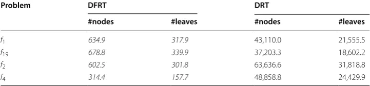
of the decision subspaces. Table 6 shows the average numbers of nodes (again inner and
leaves) and leaves. The difference of complexity is more remarkable in this case, being DRT about two orders of magnitude more complex than DFRT.
The analysis of Tables 4 and 6 highlights the capability of the DFRT learning approach
to deal with high dimensionality. Indeed, in the DFRTs generated by the learning, a rel-evant number of input variables are missing, thus proving the input variable selection implicitly performed during the regression tree learning. If, for instance we analyze the
synthetic datasets generated from f1 and f19 , we can realize that we have 1000 input
variables and, respectively, 634.9 and 678.8 nodes on average. Since the number of nodes also includes the average number of leaves, respectively 317.9 and 339.9 for the two data-sets, we have that on average the two DFRTs contain 317 and 338.9 decision nodes. This implies that at most (if a different variable is used in each decision node) 317 and 338.9 out of 1000 input variables are used on average in the DFRT. Thus, we can conclude that a relevant input variable selection is performed, since the number of nodes is lower than the number of input variables. As it occurs for all the regression decision trees, we can conclude that our approach can cope with a high number of input variables by reducing this number during the learning phase.
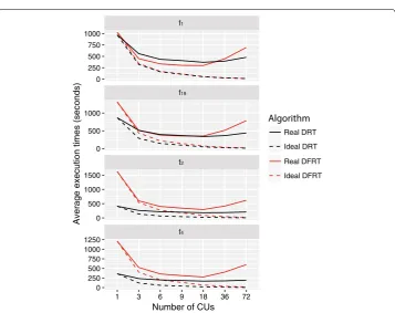
As regards scalability, we evaluate it with respect to the number of CUs and the
dimen-sionality of the datasets. Figures 5 and 6 show the average execution times (in seconds)
Table 5 Average MSEs obtained by DFRT and DRT on the training and test sets for the synthetic datasets
The best results for each dataset have been emphasized in italic font
The results have to be multiplied by 1022 , 1022 , 105 and 1033 for
f1 , f19 , f2 and f4 respectively
Problem DFRT DRT
Training Test Training Test
f1 1.5043 1.6654 2.3337 2.8851
f19 6.5671 7.3154 8.5149 12.1510
f2 3.1378 3.2097 3.8151 3.8242
f4 4.2888 4.2988 4.5396 5.3521
Table 6 Average complexity of the models obtained by DFRT and DRT for the synthetic datasets
The best results for each dataset have been emphasized in italic font
Problem DFRT DRT
#nodes #leaves #nodes #leaves
f1 634.9 317.9 43,110.0 21,555.5
f19 678.8 339.9 37,203.3 18,602.2
f2 602.5 301.8 63,636.6 31,818.8
Window8 Window9
Window6 Window7
Window4 Window5
Window2 Window3
9 18 36 72
1 3 6 1 3 6 9 18 36 72
0 200 400 600 0 250 500 750 0 300 600 900 0 500 1000 0 200 400 0 200 400 600 800 0 250 500 750 1000 0 250 500 750 1000 1250
Number of CUs
Average execution times (seconds)
Real DRT Ideal DRT Real DFRT Ideal DFRT Algorithm
Fig. 5 Average execution times of the DRT and DFRT algorithms for the real-world datasets versus the number of CUs.
f4
f2
f19
f1
1 3 6 9 18 36 72
0 250 500 750 1000 0 500 1000 0 500 1000 1500 0 250 500 750 1000 1250
Number of CUs
Average execution times (seconds)
Real DRT Ideal DRT Real DFRT Ideal DFRT Algorithm
of DFRT (red lines) and DRT (black lines) for the real world and synthetic datasets, respectively, versus the number of CUs. In the figures, we also show the ideal behavior of the two algorithms (dashed line), whose speedup is linear with respect to the number of CUs.
As we can observe, in the real datasets, DFRT is in general more time consuming, spe-cially when using a small number of CUs. However, as the number of CUs increases, both algorithms need similar computation times.
In the synthetic datasets, we can draw similar conclusions. Furthermore, we notice that, in the case of datasets with a lower number of variables, DRT is much faster than DFRT, specially when using a small number of CUs. In the case of the datasets with a higher number of variables, computation times are similar and, for some number of CUs, DFRT is faster.
There are mainly two aspects which affect the computation time. First, since the tree learning stage consists of an iterative process, the larger the number of nodes of the model, the higher the computation time. Second, the map-reduce phase searches for the best split at each iteration. This is done by analyzing all the possible splits among the candidate nodes. Hence, if the generated model is more complex, a larger number of nodes will be evaluated at each iteration with corresponding increase of the computation time. For high-dimensional datasets, DRT tends to build more complex models (a larger number of nodes) compared to DFRT, thus increasing the computation time. However, for each candidate split point, the computation of the PFGain in DFRT is much more complex than the computation of the corresponding measure in DRT and this increases drastically the computation time of DFRT with respect to DRT. Thus, in the case of data-sets with a small number of input variables, DRT is generally faster than DFRT. On the other hand, in the case of datasets with a larger number of input variables, computation times are more similar to each other and sometimes DFRT can outperform DRT (for instance, in the f1 dataset).
With respect to the number of CUs, we expect that the larger the number of CUs, the lower the computation time. However, this behavior is affected by the overhead due to communication. We can see how the ratio ideal versus real speedup is directly depend-ent on the number of CUs: the larger the number of workers, the worse the ratio. This happens because the increase of CUs requires a larger communication among workers and therefore a higher overhead, which is easily observed in the case of the synthetic datasets, where an increase in the number of CUs upon 18 requires a higher computa-tional time than using a lower number of CUs.
However, this behavior is not observed in the case of real-world problems. The reason is that the synthetic datasets have been generated uniformly over the input space, unlike the real-world problems. We observed that, in this scenario, the first phase of the dis-tributed PFV, namely the Disdis-tributed Bin Generation, tends to produce a sorted list of
bin boundaries per each variable with the maximum number of elements, namely V ·L .
of the number of nodes, the overhead due to this communication grows and makes the advantage of having a higher number of CUs ineffective.
Comparison with Distributed Random Forest
In this section, we aim to compare the results obtained by DFRT with one of the state-of-the-art algorithms available for regression problems with big data, namely DRF. We adopt DRF for two reasons. First, DRF is available in the Spark MLlib library. Second, it
has been proved that, comparing an RT versus an RF (ensemble of RTs) [41], the bias of
RF is asymptotically similar but the variance is reduced. Thus, we will compare DFRT with DRF with respect to variance, in addition to MSE (we will use the standard devia-tion to improve the readability of the results).
We execute DRF by using the default values recommended by the authors. Further-more, we have set the two parameters, which do not have default values, namely the maximum depth for any tree and the number of trees, which compose the ensemble, to
10 (parameter β ) and 20, respectively. In a preliminary experimentation, we tried
differ-ent (and larger) values for these parameters. However, we could not run the algorithm on a single CU because of memory overflow. In order to compare the algorithms under similar environments, we finally chose the previous parametrization.
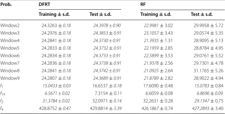
Table 7 shows the average training and test MSEs with their respective standard
devia-tions. We can observe that DFRT achieves a lower test MSE than DRF in the real world problems, while DRF obtains a lower test MSE than DFRT in the synthetic datasets. In the real datasets, we observe that RF is affected by overfitting (the test MSE is larger than almost 30% of the training MSE). However, in the case of synthectic datasets, training and test MSEs are very similar for DFRT and RF. We have applied a Wilcoxon Signed
Rank Test [46] to evaluate whether there exists a statistical difference between the two
algorithms. We adopted α=0.05 as confidence level and obtained p-value=0.1697,
which points out that there is no statistical evidence that these algorithms are different. Table 7 Average MSEs and their standard deviation obtained by DFRT and RF on the training and test sets for the real world and synthetic datasets
The best results for each dataset have been emphasized in italic font
The results have to be multiplied by 1021 , 1022 , 104 and 1031 for
f1 , f19 , f2 and f4 respectively
Prob. DFRT RF
Training ± s.d. Test ± s.d. Training ± s.d. Test ± s.d.
Window2 24.3263 ± 0.18 24.3978 ± 0.90 22.9981± 3.02 29.9958 ± 5.72
Window3 24.2976 ± 0.18 24.3853 ± 0.91 23.1057± 3.43 29.0574 ± 5.35
Window4 24.2841 ± 0.18 24.3730 ± 0.91 21.3935± 1.31 28.9095 ± 5.13
Window5 24.2833 ± 0.18 24.3732 ± 0.91 22.1959± 2.85 28.8784 ± 4.95
Window6 24.2834 ± 0.18 24.3733 ± 0.91 22.5899± 3.53 29.0761 ± 5.52
Window7 24.2836 ± 0.18 24.3738 ± 0.91 21.9378± 2.56 29.7301 ± 4.78
Window8 24.2841 ± 0.18 24.3742 ± 0.91 21.0925± 2.64 31.1765 ± 5.26
Window9 24.2807 ± 0.18 24.3689 ± 0.91 21.8789± 2.82 28.9022 ± 4.94
f1 15.0433 ± 0.03 16.6537 ± 0.18 17.6090 ± 0.48 15.0783± 0.84
f19 6.5671 ± 0.02 7.3154 ± 0.11 6.6059 ± 0.08 6.8696 ± 0.09
f2 31.3784 ± 0.02 32.0971 ± 0.14 32.2631 ± 0.28 29.1347± 0.75
As regards the standard deviation, DFRTs are characterized by smaller standard
devia-tions than DRFs, except for f19 . Moreover, the standard deviation obtained by DFRT is
small (always less than a 10% of the MSE), while in the case of RF it is greater, up to 20% in the case of real world problems. Again, we have applied a Wilcoxon Signed Rank Test
with α=0.05 . We have obtained p-value =0.0046 , thus pointing out that the standard
deviation obtained by DFRT is statistically lower than the one achieved by DRFs. This
result is very interesting, considering the observation made in [41] regarding the
vari-ance of the MSEs obtained by RFs.
Conclusions
In this work we have proposed a distributed fuzzy regression tree learning algorithm (DFRT), following the Map Reduce programming model to cope with Big Data
prob-lems. DFRT uses a novel distributed fuzzy discretizer (PFV), adapted from [38] to deal
with regression problems. PFV generates a strong fuzzy partition based on the fuzzy variance. Then, DFRT applies an iterative process to generate a binary fuzzy regression tree. The distributed version of the algorithm has been implemented using the Apache Spark framework.
We have used 8 real-world datasets, generated from the same problem. In particu-lar, all of them have the same number of instances, but they differ in the number of input variables. In addition, we have generated 4 synthetic datasets: two of them with
1000 input variables and 105 instances, and the others with 100 input variables and 106
instances. We have compared the results obtained by our approach with the distributed regression tree (DRT) and the Distributed Random Forests (DRFs) implemented in the MLlib Apache Library (included in the 1.5.2 version of the Apache Spark).
Results show that DFRT scales similar to the DRT algorithm, but the results obtained by DFRT outperform in all the cases the DRT in terms of MSE on the test set and also in terms of complexity (number of nodes and leaves). In terms of execution time, even if the scalability behavior is similar to DRT, the DFRT algorithm is slower. We have observed that, in the case of the smaller datasets (less number of features), DRT is gener-ally faster than DFRT. On the other hand, DFRT is faster (or at least similar) than DRT for the case of datasets with a large number of input variables.
As regards the comparison with DRF, the results show that DFRT and DRF are not sta-tistically different in terms of test MSE, but DFRT outperforms DRF in terms of standard deviation.
Abbreviations
CV: cross-validation; DT: decision tree; DFRT: distributed fuzzy regression tree; DRF: Distributed Random Forest; DRT: dis-tributed regression tree; FRT: fuzzy regression tree; HDFS: Hadoop Disdis-tributed FileSystem; MR: Map Reduce; MSE: mean squared error; PFV: partitioning based on fuzzy variance; RF: Random Forest; RT: regression tree.
Authors’ contributions
Authors propose a distributed fuzzy regression tree learning algorithm following the Map Reduce programming model to cope with Big Data problems. Authors adapt a novel distributed fuzzy discretizer (PFV) from [38] to deal with regres-sion problems. The algorithm has been implemented using the 1.5.2 verregres-sion of Apache Spark framework. All authors read and approved the final manuscript.
Author details
Acknowlegements
The authors would like to acknowledge Dr. Armando Segatori for the precious suggestions and explanations on the implementation of the distributed fuzzy decision trees for big data classification problems.
Competing interests
The authors declare that they have no competing interests.
Availability of data and materials
Real world datasets can be downloaded from the website http://ico2s.org/datasets/psp_benchmark.html. To download the synthetic datasets, please contact the corresponding author Javier Cózar [email protected].
Funding
This work has been partially supported by the project PRA 2017 “IoT e Big Data: metodologie e tecnologie per la raccolta e l’elaborazione di grosse moli di dati”, funded by the University of Pisa. This work has been partially funded by the Span-ish Research Agency (AEI/MINECO) and FEDER (UE) through projects TIN2013-46638-C3-3-P and TIN2016-77902-C3-1-P. This work has been partially funded by the Junta de Comunidades de Castilla-La Mancha and FEDER (UE) funds through project SBPLY/17/180501/000493. Javier Cózar has also been funded by the MICINN grant FPU12/05102.
Publisher’s Note
Springer Nature remains neutral with regard to jurisdictional claims in published maps and institutional affiliations.
Received: 22 August 2018 Accepted: 29 November 2018
References
1. Arana-Daniel N, Gallegos AA, López-Franco C, Alanís AY, Morales J, López-Franco A. Support vector machines trained with evolutionary algorithms employing kernel adatron for large scale classification of protein structures. Evol Bioinform. 2016;12:285–302.
2. Bacardit J, Krasnogor N. The icos psp benchmarks repository; 2008. http://ico2s .org/datas ets/psp_bench mark.html. Accessed 3 Dec 2018.
3. Berzal F, Cubero JC, Marın N, Sánchez D. Building multi-way decision trees with numerical attributes. Inf Sci. 2004;165(1):73–90.
4. Breiman L. Random forests. Mach Learn. 2001;45(1):5–32.
5. Breiman L, Friedman JH, Olshen RA, Stone CJ. Classification and regression trees. Monterey: Wadsworth & Brooks; 1984.
6. Cheng HD, Chen JR. Automatically determine the membership function based on the maximum entropy principle. Inf Sci. 1997;96(3–4):163–82.
7. Cózar J, delaOssa L, Gámez JA. Learning tsk-0 linguistic fuzzy rules by means of local search algorithms. Appl Soft Comput. 2014;21:57–71.
8. Cózar J, delaOssa L, Gámez JA. Tsk-0 fuzzy rule-based systems for high-dimensional problems using the apriori principle for rule generation. In: Rough sets and current trends in computing, lecture notes in computer science, vol 8536. New York: Springer International Publishing; 2014. p. 270–9.
9. Dean J, Ghemawat S. Mapreduce: simplified data processing on large clusters. Commun ACM. 2008;51(1):107–13. 10. Slowiński R. Fuzzy sets in decision analysis, operations research and statistics, vol 1. US: Springer; 2012.
11. Diao R, Sun K, Vittal V, O’Keefe RJ, Richardson MR, Bhatt N, Stradford D, Sarawgi SK. Decision tree-based online volt-age security assessment using pmu measurements. IEEE Trans Power Syst. 2009;24(2):832–9.
12. Dubois D, Prade H. Unfair coins and necessity measures: towards a possibilistic interpretation of histograms. Fuzzy Sets and Systems. 1983;10(1–3):15–20.
13. Fonarow GC, Adams KF, Abraham WT, Yancy CW, Boscardin WJ, Committee ASA. Risk stratification for in-hospital mortality in acutely decompensated heart failure: classification and regression tree analysis. JAMA. 2005;293(5):572–80.
14. Franklin J. The elements of statistical learning: data mining, inference and prediction. Math Intell. 2005;27(2):83–5. 15. Garcia S, Luengo J, Sáez JA, Lopez V, Herrera F. A survey of discretization techniques: taxonomy and empirical
analy-sis in supervised learning. IEEE Trans Knowl Data Eng. 2013;25(4):734–50.
16. Goetz T. The decision tree: taking control of your health in the new era of personalized medicine. Emmaus: Rodale; 2010.
17. Gupta A, Mehrotra KG, Mohan C. A clustering-based discretization for supervised learning. Stat Probab Lett. 2010;80(9):816–24.
18. Haskell RE. Regression tree fuzzy systems. In: Proceedings of the ICSC symposium on soft computing, fuzzy logic, artificial neural networks and genetic algorithms, University of Reading, Whiteknights, Reading, England; 1996. p. 26–8.
19. Hastie T, Tibshirani R, Friedman J. The elements of statistical learning: data mining, inference, and prediction. Springer series in statistics, vol 10, 1st ed. New York: Springer; 2001.
20. Izrailev S, Agrafiotis D. A novel method for building regression tree models for qsar based on artificial ant colony systems. J Chem Inf Comput Sci. 2001;41(1):176–80.
21. Keller JM, Gray MR, Givens JA. A fuzzy k-nearest neighbor algorithm. IEEE Trans Syst Man Cybern. 1985;4:580–5. 22. Kim H, Loh WY. Classification trees with unbiased multiway splits. J Am Stat Assoc. 2001;96(454):589–604. 23. Kotsiantis S, Kanellopoulos D. Discretization techniques: a recent survey. GESTS Int Trans Comput Sci Eng.
24. Leathwick J, Elith J, Francis M, Hastie T, Taylor P. Variation in demersal fish species richness in the oceans surrounding new zealand: an analysis using boosted regression trees. Mar Ecol Prog Ser. 2006;321:267–81.
25. Leskovec J, Rajaraman A, Ullman JD. Mining of massive datasets. Cambridge: Cambridge University Press; 2014. 26. Leskovec J, Rajaraman A, Ullman JD. Mining of massive datasets. Cambridge: Cambridge university press; 2014. 27. Liu H, Hussain F, Tan CL, Dash M. Discretization: an enabling technique. Data Mining Knowl Discov.
2002;6(4):393–423.
28. Maciel AI, Costa IG, Lorena AC Measuring the complexity of regression problems. In: 2016 international joint confer-ence on neural networks (IJCNN). New York: IEEE; 2016. p. 1450–7.
29. Medasani S, Kim J, Krishnapuram R. An overview of membership function generation techniques for pattern recog-nition. Int J Approx Reason. 1998;19(3–4):391–417.
30. Meng X. Mllib: Scalable machine learning on spark. In: Spark Workshop April; 2014.
31. Mori H, Kosemura N, Ishiguro K, Kondo T. Short-term load forecasting with fuzzy regression tree in power systems. In: 2001 IEEE international conference on systems, man, and cybernetics, vol 3. New York: IEEE; 2001. p. 1948–53. 32. Nieradka G, Butkiewicz B. A method for automatic membership function estimation based on fuzzy measures. In:
International fuzzy systems association world congress. Berlin: Springer; 2007. p. 451–60
33. Olaru C, Wehenkel L. A complete fuzzy decision tree technique. Fuzzy Sets Syst. 2003;138(2):221–54. 34. Pedrycz W. Why triangular membership functions? Fuzzy Sets Syst. 1994;64(1):21–30.
35. Prasad AM, Iverson LR, Liaw A. Newer classification and regression tree techniques: bagging and random forests for ecological prediction. Ecosystems. 2006;9(2):181–99.
36. Quinlan RJ. Learning with continuous classes. In: 5th Australian joint conference on artificial intelligence. Singapore: World Scientific; 1992. p. 343–8.
37. Segal MR. Regression trees for censored data. Biometrics. 1988;44:35–47.
38. Segatori A, Marcelloni F, Pedrycz W. On distributed fuzzy decision trees for big data. IEEE Trans Fuzzy Syst. 2018;26(1):174–92.
39. Suárez A, Lutsko JF. Globally optimal fuzzy decision trees for classification and regression. IEEE Trans Pattern Anal Mach Intell. 1999;21(12):1297–311.
40. Tang K, Li X, Suganthan PN, Yang Z, Weise T. Benchmark functions for the cec2010 special session and competition on large-scale global optimization. Tech. rep. nature inspired computation and applications laboratory; 2009. 41. Wager S Asymptotic theory for random forests. arXiv preprint; 2014. arXiv :14050 352.
42. Ward JS, Barker A. Undefined by data: a survey of big data definitions. arXiv preprint; 2013. arXiv :13095 821. 43. Weber R. Fuzzy-id3: a class of methods for automatic knowledge acquisition. In: Proceedings of the 2nd
interna-tional conference on fuzzy logic and neural networks; 1992.
44. Westhead DR, Thornton JM. Protein structure prediction. Curr Opin Biotechnol. 1998;9(4):383–9. 45. White T. Hadoop: the definitive guide. Sebastopol: O’Reilly Media, Inc.; 2012.
46. Wilcoxon F. Individual comparisons by ranking methods. Biometrics Bull. 1945;1(6):80–3. 47. Yuan Y, Shaw MJ. Induction of fuzzy decision trees. Fuzzy Sets Syst. 1995;69(2):125–39. 48. Zaharia M. Apache Spark MLlib; 2009. http://spark .apach e.org/mllib /. Accessed 26 Sept 2017.
49. Zaharia M, Chowdhury M, Franklin MJ, Shenker S, Stoica I. Spark: cluster computing with working sets. HotCloud. 2010;10(10–10):95.
50. Zeinalkhani M, Eftekhari M. Fuzzy partitioning of continuous attributes through discretization methods to construct fuzzy decision tree classifiers. Inf Sci. 2014;278:715–35.
51. Zhang Y, Skolnick J. The protein structure prediction problem could be solved using the current pdb library. Proc Natl Acad Sci. 2005;102(4):1029–34.