Using deep learning for short text
understanding
Justin Zhan
*and Binay Dahal
Introduction
As we move towards the micro blogging era, and with the ever-growing presence of digi-tal news, delivering the relevant content to the right users based on the limited context information present in short texts has become more important than ever. For example, let’s take twitter, where the character limit per tweet is a mere 140 characters. Display-ing ads relevant to a particular user requires understandDisplay-ing what type of tweet she/he generally produces. If the user generally tweets about sports, it is more appropriate if sports related ads are shown to their timeline. Other areas where short texts are used are web queries, news recommendations based on news titles, etc. These all require under-standing short texts and delivering the right content. However, underunder-standing short texts involves confronting many challenges that make the task difficult. Short texts like web queries and tweets generally lack proper syntactic formation. Unlike in longer docu-ments, there is a dearth of enough statistical information in those short texts. Also, short texts with similar meaning may not share any common words between them. For exam-ple, lets take two short texts, “new version of windows OS” and “upcoming Operating System from Microsoft”. The given short texts don’t share any keywords between them, but we know that these two are related. These factors make understanding short text a
Abstract
Classifying short texts to one category or clustering semantically related texts is chal-lenging, and the importance of both is growing due to the rise of microblogging platforms, digital news feeds, and the like. We can accomplish this classifying and clustering with the help of a deep neural network which produces compact binary rep-resentations of a short text, and can assign the same category to texts that have similar binary representations. But problems arise when there is little contextual information on the short texts, which makes it difficult for the deep neural network to produce similar binary codes for semantically related texts. We propose to address this issue using semantic enrichment. This is accomplished by taking the nouns, and verbs used in the short texts and generating the concepts and co-occurring words with the help of those terms. The nouns are used to generate concepts within the given short text, whereas the verbs are used to prune the ambiguous context (if any) present in the text. The enriched text then goes through a deep neural network to produce a prediction label for that short text representing it’s category.
Keywords: Short text classification, Semantic enrichment, Deep neural network
Open Access
© The Author(s) 2017. This article is distributed under the terms of the Creative Commons Attribution 4.0 International License (http://creativecommons.org/licenses/by/4.0/), which permits unrestricted use, distribution, and reproduction in any medium, provided you give appropriate credit to the original author(s) and the source, provide a link to the Creative Commons license, and indicate if changes were made.
RESEARCH
challenging task. To identify the relatedness of these texts, we need to find common con-cepts between them.
Finding concepts of words from the given short text and identifying the words that occur frequently with those words are collectively represented as semantic enrichment. Mapping of words into their concepts is an important task in understanding natural language. As we can see, concepts are the medium which glue terms that are not related syntactically to a common ground. For example, the terms “apple” and “orange” are not related syntactically but both of those terms can be glued by the concept “fruit”. Hence, finding the most appro-priate concept of any given word is the main task in conceptualization. There is a challenge that is very hard to solve in conceptualization, which is the context sensitive nature of word to concept mapping. For instance, we can see the context of the word “apple” is “fruit” or “food” when it is used with words like “orchard” or “tree”. But the same word “apple” has the context of “company” or “firm” when it is used with “ipad”, “iphone” or some other technological terms. There are many approaches proposed to solve or mitigate this prob-lem. One of them does this with a simple two-stage solution combining a topic model and a probabilistic knowledge base such that we can consider both semantic relationships among words for modeling the context, and conceptual relationships between words and concepts for mapping the words to concepts within the given context [1].
Use of universal probabilistic semantic networks like Probase to enrich the text adds far more context and meaning, enabling for better classification. However, there are many cases when using just the noun terms of a short text to generate concepts is not sufficient to clearly identify the context of those texts. This is especially true for ambigu-ous short texts. Let us take for example two short texts: “five people hospitalized by eat-ing poisonous apple” and “two people imprisoned for hackeat-ing into apple”. Here, useat-ing just the noun terms generates the same concepts for both the texts, as both of them con-tain the noun terms “people and apple” but the context of these two texts are completely different. The context of those texts will be clear if we consider the verbs “eating” and “hacking” from the respective texts. Let us look at another example, “United defeated by City 2-1”. In this text, if we take the noun term only we cannot figure out its context properly. But if we take into consideration the verb “defeated”, we may get the sense that it is talking about a sporting events. It can also be showed that the adjectives used in the text also help to disambiguate it for higher accuracy in classification.
Our contribution through this paper will be generating richer concepts for a short text, considering the verbs in addition to the nouns present in the text, hence adding more precise features to the text. These added features generated from verbs help to remove ambiguity if any, present in the text that could not be removed through the concepts generated by the noun terms only. We then present a simple four layers deep neural net-work which takes the enriched text as input and classify it into one of the categories.
Related works
Then various approaches came for enriching short texts that used domain-specific information. One of the approaches is to treat the short text as a web query and enrich the given text with the results from the search engine to that query (e.g titles of web page and snippets) [8–10]. This method takes advantage of variety of web documents to identify the appropriate context. Another effective approach used external knowledge base such as WordNet [11, 12], Wikipedia [13, 14], the Open Directory Project (ODP) [15] etc. to enrich the given short text. As Gabrilovich [14] has demonstrated, there is value in using Wikipedia as an additional source of features for text categorization and determining the semantic relatedness between texts. The open editing policy of Wikipe-dia yields amazing quality. A recent study [16] found Wikipedia accuracy to rival that of Britannica. Substantial works have been conducted in automatic web query classifica-tion. One of them is web query classification using labeled and unlabeled training data [17]. Another approach for web query classification uses machine learning techniques in an automatic classifier to categorize queries by geographical locality [18]. Query type classification for web document retrieval is another related work [19].
Apart from enriching the given short texts, work has been done to extract efficient representations of those texts so as to perform information retrieval or classification. Recently, Salakhutdinov and Hinton [20] have proposed semantic hashing which is a novel information retrieval mechanism. In this model, we stack RBMs [21] which learns the document representation through a compact binary code. The semantic of a docu-ment is supposedly captured by the code.
The approaches mentioned above can produce satisfactory result to some extent, but they each have their own limitations. Treating a short text as search query may work well for popular queries but for unpopular queries, the search engine will most likely return some irrelevant results which acts as a noise to the short query instead of enriching it. Enriching a short text with the information obtained from WordNet also has its prob-lems. Although WordNet contains information about general terms, it does not contain information for proper nouns such as “USA” or “Microsoft”. Also, it does not weigh the senses based on the frequency of their usage. There is another approach to semantic enrichment which uses Probase for enriching the given short text [22]. Probase [1, 23, 24] is a large collection of worldly concepts and their likely instances presented in proba-bilistic form. It contains about millions of such concepts and instances. The basic idea is to extract the noun terms from the given short text and perform a lookup into Probase to generate multiple concepts that relate to those noun terms. We can also extract occurring terms from Probase for those noun terms. Then, these concept terms and co-occurring terms [22] along with those noun terms form the enriched short text. This approach produces by far the best classification result over other previous works.
Preliminaries
which captures the abstract relationships among different features of data hierarchically and an auto-encoder, one of the unsupervised deep learning algorithm.
Probase
Probase [23] is a very large network of millions of concepts where the semantic entities are quantified by probabilistic method. These concepts are obtained by mining the web-pages which contain it. It basically works by matching the patterns in it’s syntax. Concepts are further enriched by its instances and attributes using relationships like “is a”, “has a” etc. For example, apple and orange are two of the most used instances of concept fruit. Such concepts and instances are quantified in Probase by probability score of having t as a instance given c as a concept: p(t|c). Given all the concepts, p(c|t) is the probability of concept c provided instance c, which is also contained in Probase. In addition, Probase gives p(t1|t2), the probability of co-occurring two instances t1 and t2. Probase also contains numerous other scores and probabilities. This abundant probability information among concepts and instances allows us to provide additional context in text understanding.
VerbNet
This is the manually constructed list of verbs that represents the categories of short text we are considering. In this paper, we have considered news titles from the dataset of our experiment as short texts. As our dataset contains news titles from seven categories, our extracted verbs fall in one of those categories. So we compiled a list of 160 verbs that somewhat represents any of those categories. For example, a verb like play, win or lose can represent the football news category, while verbs like endanger and protect can rep-resent environment category.
For each category, verbs are extracted from the news title and are sorted in terms of their frequency. While doing so, the common verbs like ‘come’, ‘look’, ‘see’ etc. are ignored. Auxiliary verbs are not taken into consideration too, as they are insignificant to the classification task. From each of the compiled lists of frequently occurring verbs, around 20 most frequent verbs are selected and inserted to the semantic vocabulary. This enabled each of those frequently occurring verbs to be features of short text based on which classification is done. We experimented with different verbs size from each category but the improvement was insignificant as verbs size was increased. The optimal verbs size from each category was fixed to 20.
Backpropagation
These back propagated error values are used to compute the gradient descent [27] of the loss function. We apply some weight update rule based on the gradient descent of loss function to optimize the weight of the network and hence, train the network to learn the function required to describe the input examples.
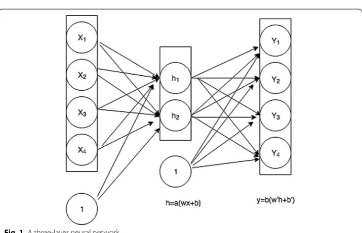
In Fig. 1, we show a simple neural network with three layers. First layer is L1 which consists of four nodes. Second is the hidden layers with two nodes represented by L2 and last one is an output layer with four nodes each representing a component of output. The nodes in hidden layer and output layer can be activated by same function or differ-ent ones. We have shown two functions α and β acting on these layers. If i is an arbitrary
node in a certain layer and j is a node that connects its output to it, then we can repre-sent the weight from jth node in previous layer to ith node in next layer by wij.
If we take squared error as the error function, which is given as:
where E is the squared error, h is the estimated output from the network, and y is the actual output.
For each neuron j in the network, its output is:
where α is the differentiable and non-linear activation function. Sigmoid function is the
commonly used such function. E= 1
2(h−y) 2
aj=α(zj)=α n
i=1
wijai
α(z)= 1 1+e−z
We can apply following chain rule to compute the descent of error with respect to each weight of the network.
Applying some calculus, we can find
where, δj= ∂aj∂Eα′(zj).
Deep neural network and autoencoder
Deep neural network is simply a neural network with multiple hidden layers. Due to this multiple hidden layers, it can effectively represent any complex input in a hierarchical abstraction. But simply training a deep network with backpropagation to compute the gra-dient of error will not produce good result. In some cases, the results are even worse than the network with single hidden layers. This lack of progress using deep networks can be mainly attributed to vanishing gradient problem or exploding descent problem. What these mean is that due to the random initialization of weights and backpropagating errors one layer at a time, the weights learn at different speeds. Specifically, as we go backwards from output layer weights learn at decreasing speed. Or sometimes, weights learn very much faster as we go backwards. Either way, the gradient of weights are unstable. This is the main reason for deep networks to get stuck at learning as we increase the hidden layers.
The effective solution to this obstacle in training deep network was first proposed by Hinton [28]. It applied greedy layer by layer pre-training of the layers in unsuper-vised fashion. What it does is adjusts the weight of the network to the comparable value instead of feeding inputs to network with randomly generated weights. Then, in second stage, supervised training is performed with the labeled data to fine tune the weights. Hence, deep neural networks trained in this way can effectively find the optimal repre-sentation of the network parameters.
An autoencoder is one of the deep learning algorithm which is basically a three layer neural network that tries to reconstruct the input with minimal error. Figure 1 depicts the working of an autoencoder. The network takes an input and constructs a hidden representation through hidden layer. This is an encoding phase. The output layer just tries to reconstruct the input so the hidden representation can be taken as a code to the original input. Input reconstruction is the decoding phase. This process is completely unsupervised.
Formally, an autoencoder takes an input x∈ [0, 1]d and encodes it to the hidden repre-sentation h∈ [0, 1]d′ through some mapping function s.
where s is any mapping function like sigmoid and W and b are the weight and bias from input to hidden layer. The latent code h is then mapped back in the form of y which is the reconstruction of original input x. y has the same size as x.
∂E ∂wij
= ∂E
∂aj
∂aj
∂zj
∂zj
∂wjk
∂E
∂wij =δjai
h=s(Wx+b)
where W′ and b′ are weights and bias from hidden to output layer. The reconstruction error can be measured with one of the loss functions. The squared loss error and cross entropy error is given below. Any one of them can be used.
The approach
To start with, first we describe the following phrases used in our system:
• Semantic features Every noun and verb terms from the input short text, concepts representing them, and co-occurring terms constitutes the Semantic features. This is the result for any given short text after we perform co-occurring phase.
• Semantic vocabulary A list of top-k(eg-3000) semantic features that occurs in highest frequency in our training dataset.
• Semantic feature vector For each enriched input short texts, a fixed sized vector (equal to the size of vocabulary) where each position gives the count of semantic fea-ture present in it.
Now let us consider our dataset contains n training examples (short texts). After enrichment with noun and verb terms, we represent those short texts as: XE =x1,x2,x3, ...,xn∈Rk∗n as described above, where k is the feature vector dimension.
The position of the semantic feature is used to identify each row of feature vector. Here, xij represents the number of times feature j occurs in the enriched short text i. Our main aim is to learn the correct category of the provided input short text and output the label Y corresponding to that category.
To get enriched text XE from input text X, it first goes through pre-processing,
con-ceptualization and co occurrence phase.
Our proposed solution to the problem defined above is sketched in algorithmic view below:
Algorithm 1 outlines the pre-processing of the input text. The first step in pre-process-ing is to remove the punctuation from the input text. Then it extracts the noun terms
L(xz)= ||x−y||2
L(x,z)= − d
k=1
and stores them in a list. Similarly, it extracts Verb terms from input text and stores them in a separate list. For each noun in Noun list, if PROBASE contains it then add those terms to a pre-processed list. It does the same for each of the verb terms, but it looks into VERBNET instead of PROBASE. This algorithm has the run time complexity of O(n) as each operation of removing punctuation and extracting noun and verb terms depends linearly on the size of the input.
Algorithm 2 takes the output from algorithm 1 as input and performs conceptualiza-tion. For each term in its input, algorithm 2 performs the look-up into PROBASE to find n relevant concepts for the term and adds those concepts along with the terms in the conceptualization list. Algorithm 2 also prunes the irrelevant concepts gathered from PROBASE. We talk about this in detail in the upcoming section. The run time complex-ity of this algorithm is O(n) as the loop runs for n times which is the size of input.
This algorithm finds the co-occurring terms of the output terms from the concep-tualization algorithm. For each term in its input, it finds top m relevant co-occurring terms. Again, PROBASE is used to find the terms. These generated co-occurring terms are stored in a list along with the terms from previous algorithms. Some filtering of irrel-evant terms is done which is described in the next section. It runs on O(n) as well.
Algorithm 4 is concerned with predicting the correct category of input short text. After an input text goes through all of the previous algorithms, it is represented in vec-tor form, normalized and then fed to our deep neural network model. The model then returns the prediction for the input text.
Enrichment and classification flow
the classification phase classifies the enriched text to a certain category. Hence, our pro-posed system contains mainly two modules: the enrichment module and classification module. First we describe the enrichment module, and then the classification module in a later sub-section:
Let X be the input short text which first goes through the enrichment phase.
Pre‑processing
We extract noun and verb terms from X. So new representation of X is:
Xp=x1,x2,x3,. . .,xk, where xi, 1≤ i≤k is the extracted noun, or verb terms of X.
While pre-processing the given input text, we consider the longest phrase that is con-tained in PROBASE. For example, in short text “New York Times Bestseller”? although New York is a noun term in itself, we take “New York Times”? as a single term. We need to remove stopwords and perform word stemming, before parsing such terms.
Conceptualization
We enrich XP obtained from pre-processing by finding the concepts of all the xi in XP
with the help of probase and our manually built verb network which further adds news features to XP. It is just a lookup operation in the networks which generates the ranked
list of concepts which relate to the xi in XP. We denote the result of this phase by XC:
XC =x1,x2,x3, ...,xm.
Where xi, 1≤i≤m are the union of terms from XP and the terms obtained from
con-ceptualization and m > k. There are cases when irrelevant concepts of given terms can appear in this phase. For instance, given a short text “apple and microsoft”? a concept like “fruit”? may appear, which is irrelevant in this context. So we apply following mecha-nism to remove such ambiguity.
Mechanism In case of ambiguity of two or more concepts given the terms, we can employ a simple Naive Bayesian mechanism proposed by Song et al. [10]. It estimates the posterior probabilities of each concepts given the instances. As a result, most com-mon concepts associated with the instances get higher posterior probability. The prob-ability of a concept is given formally c as:
which is proportional to: p(c)M
i p(ei|c).
Using this, given a short text “apple and microsoft”?, we can get the higher posterior probabilities for concepts like “corporation”, “IT firm” etc. whereas irrelevant concept like “fruit” gets lower probability and hence pruned.
Co‑occurring terms
We take the result from previous phase and enrich it using the co-occurring terms. The result of this is the finally enriched version of the original short text which is given by:
where xi, 1≤i≤n are the union of terms from XC and the terms obtained from this
phase and n > m.
(1)
p(c|E)= p(E|c)p(c)
p(E)
(2)
Co-occurrences give the important information to understand the meaning of words. These are the words that frequently co-occur with the original terms. We know from Distributional hypothesis [29] “words that occur in the same context tend to have similar meanings”.
To find the co-occurring words, we take the terms obtained from the pre-processing phase, and enrich with terms that frequently co-occur with these terms. For each origi-nal term, we look into probase to find the co-occurring terms.
DNN model
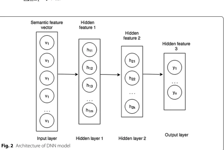
We designed a four layer deep neural network as the learning element for our input text. It was trained in semi-supervised fashion as we discussed earlier. It is as shown in Fig. 2.
Each layers except the input layer shown in the figure, are pre-trained with an auto-encoder. This is done in layer by layer fashion. To pre-train the first hidden layer, we train an auto-encoder with input layer and hidden layer same as in Fig. 2. The output layer tries to reconstruct the original input. Once this is done, we pre-train second den layer with separate auto-encoder. This auto-encoder has the previously trained hid-den layer as its input and tries to generate code for its input. All subsequent layers are pre-trained in same manner. We used sigmoid as activation function and cross-entropy error as defined above for loss function. Through this pre-training, the parameters of our network achieve some nearly optimal value.
The pre-training phase alone can not optimize the network parameters completely although they can attain some good values. So we perform supervised fine-tuning to our pre-trained network. Fine-tuning process is as shown in Fig. 3.
We feed our DNN model with a feature vector that represents our short text through input layer. To correctly predict the category, we add softmax layer to our pre-trained network. Output oi for any node i is computed as:
oi= nexp(ai) m=1exp(am)
,
where n is the total nodes on softmax layer. Output from this network is the predic-tion class for the given input vector. As shown above, our DNN model goes through two training stages. First is unsupervised pre-training and then the supervised fine-tuning [30].
Experiment
For short text understanding, we experimented with the task of classifying news titles into categories. We used news titles as the short text and classified them into specific categories.
Data set
We extracted the news titles from the Guardian web site for our classification purpose. We used seven different data sets which include news titles from seven categories. The seven categories were World News, Football news, Tech news, Art and Entertainment news, Business News, Environment news and Travel news. For each category, there were 7000 news titles as training data and 1000 news titles as test data. So we performed our experiment on altogether 49,000 training data and 7000 test data.
Feature vocabulary creation
The first task was to create a feature vocabulary out of the obtained dataset. This feature vocabulary is the list of 3000 most frequently occurring concepts from all of the dataset. We passed each news title from dataset through pre-processing, conceptualization, and co-occurring terms phase and sorted a list of 3000 most frequently occurring concepts or terms.
Input representation
After feature vocabulary was constructed, the next task was to represent each input short text (news title) into a vector form that can be fed into our deep neural network.
For this, we passed each text through all the phases and generated their relevant con-cepts and co-occurring terms. Input representation of a given short text is the 3000 dimensional vector, where ith row of this vector represents the frequency of ith item of feature vocabulary in this enriched short text.
Deep neural network training and evaluation
We used the DNN model as described above for the training purpose (both pre-train-ing and fine tunpre-train-ing). At first, all the parameters of the network, that is the weights and biases, are randomized using Gaussian distribution. To update these parameters we used mini-batches gradient descent technique. The size of batches for pre-training and fine tuning are 100 and 500 respectively. Instead of updating the parameters after every train-ing examples (stochastic gradient descent) or updattrain-ing the parameters once after all the training examples have been processed (batch gradient descent), this technique speeds up the training process as gradient of loss is averaged over each mini-batch (Table 1).
In this research, our DNN has a size of 3000, 500, 250 and 128 i.e. input layer has 3000 elements and sub-sequent hidden layers are of 500, 250 and 128, sizes. The model parameters like number of units in hidden layers, batch size etc. are set based on the result of validation set.
Result
Table 1 shows the classification accuracy of various methods applied to “Wikipedia Short Sentences” dataset as stated in [22]. We wanted to see the effect of adding verb terms in overall accuracy. So we re-implemented the EDNN-SVM done in [22] and tested with our dataset. In our work, we call SVM method applied to our dataset as EDNN-N as it uses just the noun terms for enrichment. The accuracy of this experiment was 58.02%.
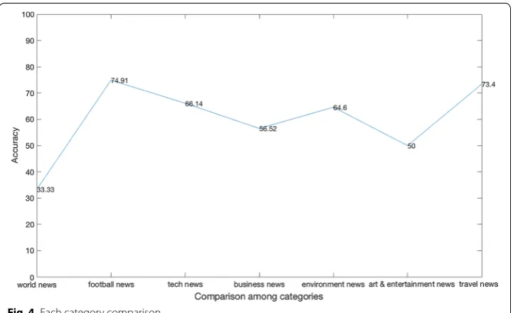
After that, we included the verb terms along with noun terms and noun phrases in fea-ture vocabulary as well as feafea-ture vector and conducted the experiment to see if inclu-sion of verb terms can remove the ambiguity (if any) and improve the accuracy of the result. We call this EDNN-NV model. The accuracy obtained was 60.25%. So there was about 2% increase in accuracy after considering verb terms present in a given short text. Figure 4 shows the accuracy of each category predicted by our model EDNN-NV. We have a lowest accuracy for World News category which is 33.33%. Similarly, we have highest accuracy for Football News category which is 74.91%. The other five categories
Table 1 Comparison among various classification methods [22]
Method Enriched method Input representation Accuracy (%)
OS-SVM Not enriched 3000D semantic feature vectors 29.00
CACT-SVM CACT 3000D semantic feature vectors 47.52
WordNet-SVM WordNet-based 3000D semantic feature vectors 36.15 Wiki-SVM Wikipedia-based 3000D semantic feature vectors 39.06
EDNN-SVM CACT Learned 128D binary code vectors 51.35
have accuracy in between these percentages. Figure 5 compares the results of EDNN-N and our EDNN-NV model
Conclusions
Our research tackled the problem of classifying short texts. The challenge of short texts are lack of enough context and the ambiguity that may arise due to it. So, we imple-mented the conceptualization and co-occurring terms enrichment technique in our work, for a given short text and presented a novel idea of including verb terms in text enrichment. First, we computed the sorted list of verbs occurring in the dataset and fil-tered the list with the verbs that somewhat represent the categories we had considered. Then, we inserted those filtered verbs into the previously computed feature vocabulary.
Fig. 4 Each category comparison
This way, the representative verbs become the feature for incoming short text. We also presented a simple four layers deep neural network to classify the input short text.
Hence, our research shows that albeit low, the inclusion of verb terms in addition to noun terms helps to improve the classification of short text. Although the size of Verb-Net is relatively smaller and just contains the representative verb in the dataset, it can be scaled up by mining the web. Through this work, we just wanted to show that verb terms can help improve the short text classification. This paves a way for considering other parts of speech like Adjectives to be included for classification.
Authors’ contributions
BD performed the literature review, implemented the proposed algorithm and conducted the experiments. JZ advised BD all aspects of the paper development. Both authors read and approved the final manuscript.
Authors’ information
Binay Dahal is a graduate student with the Department of Computer Sciences, University of Nevada Las Vegas. His research interests include Big Data Analytics, Text Analysis, and Imaging Analysis. Justin Zhan is the director of Big Data Lab , Department of Computer Science, at Howard R. Hughes College of Engineering, University of Nevada, Las Vegas. His research interests include Big Data, Information Assurance, Social Computing, and Health Science. He is a steering chair of AS E/IEEE International Conference on Social Computing (SocialCom), ASE/IEEE International Conference on Pri-vacy, Security, Risk and Trust (PASSAT), and ASE/IEEE International Conference on BioMedical Computing (BioMedCom). Currently, he is editor-in-chief of the International Journal of Privacy, Security and Integrity, International Journal of Social Computing, and Cyber-Physical Systems, and a managing editor of SCIENCE journal and HUMAN journal. He has served as a conference general chair, a program chair, a publicity chair, a workshop chair, or a program committee member for 160 international conferences and editor-in-chief, editor, associate editor, guest editor, editorial advisory board member, or editorial board member for 30 journals. He has published 200 articles in peer-reviewed journals and conferences, and delivered above 30 keynote speeches and invited talks. He has been involved in a number of projects as a PI or a Co-PI, funded by the National Science Foundation, the U.S. Department of Defense, National Institutes of Health, among other agencies.
Acknowledgements
We gratefully acknowledge the United States Department of Defense (W911NF-17-1-0088, W911NF-16-1-0416), AEOP/ REAP programs support, the National Science Foundation (1625677, 1710716), and the United Healthcare Foundation (UHF #1592) for their support and finance for this project.
Competing interests
The authors declare that they have no competing interests. Availability of data and materials
Not applicable. Consent for publication Not applicable.
Ethics approval and consent to participate Not applicable.
Funding Not applicable.
Publisher’s Note
Springer Nature remains neutral with regard to jurisdictional claims in published maps and institutional affiliations.
Received: 23 June 2017 Accepted: 6 October 2017
References
1. Kim D, Wang H, Oh A.H. Context-dependent conceptualization. In: Proceedings of 23rd international joint confer-ence artificial intelligconfer-ence; 2013. p. 2654–2661.
2. Lenat DB, Davis R. Knowledge-based systems in artificial intelligence. New York: McGrav-Hill. Nev; 1982. 3. Lenat DB, Guha RV. Building large knowledge-based systems; representation and inference in the Cyc project.
Boston: Addison-Wesley Longman Publishing Co., Inc.; 1989.
4. Baeza-Yates R, Ribeiro-Neto B. Modern Information Retrieval. New York: ACM Press; 1999.
6. Budanitsky A, Hirst G. Evaluating wordnet-based measures of lexical semantic relatedness. Comput Linguist. 2006;32(1):13–47.
7. Jarmasz M. Roget’s thesaurus as a lexical resource for natural language processing. arXiv preprint arXiv:1204.0140. 2012.
8. Sahami M, Heilman TD. A web-based kernel function for measuring the similarity of short text snippets. In: Proceed-ings of 15th international conference world wide web; 2006. p. 377–86.
9. Yih WT, Meek C. Improving similarity measures for short segments of text. In: Proceedings of 22nd national confer-ence artificial intelligconfer-ence; 2007. p. 1489–94.
10. Shen D, Pan R, Sun J-T, Pan JJ, Wu K, Yin J, Yang Q. Query enrichment for web-query classification. ACM Trans Inf Syst. 2006;24(3):320–52.
11. Fellbaum C. Wordnet: an electronic lexical database. IEEE Trans Knowl Data Eng. 2016;28(2):566–79.
12. Hu X, Sun N, Zhang C, Chua T.-S. Exploiting internal and external semantics for the clustering of short texts using world knowledge. In: Proceedings of 18th ACM conference information knowledge manage; 2009. p. 919–28. 13. Banerjee S, Ramanathan K, Gupta A. Clustering short texts using wikipedia. In: Proceedings of 30th annual
interna-tional ACM SIGIR conference research and development information retrieval; 2007. p. 787–88.
14. Gabrilovich E, Markovitch S. Computing semantic relatedness using wikipedia-based explicit semantic analysis. In: Proceedings of 20th international joint conference artificial intelligent; 2007. p. 1606–11.
15. Gabrilovich E, Markovitch S. Feature generation for text categorization using world knowledge. In: Proceedings 19th international joint conference artificial intelligence; 2005. p. 1048–53.
16. Giles J. Internet encyclopaedias go head to head. Nature. 2005;438(7070):900–1.
17. Beitzel SM, Jensen EC, Frieder O, Grossman D, Lewis DD, Chowdhury A, Kolcz A. Automatic web query classification using labeled and unlabeled training data. In: Proceedings of the 28th annual international ACM SIGIR conference on research and development in information retrieval. New York: ACM; 2005. p. 581–82.
18. Gravano L, Hatzivassiloglou V, Lichtenstein R. Categorizing web queries according to geographical locality. In: Proceedings of the twelfth international conference on information and knowledge management. New York: ACM; 2003. p. 325–33.
19. Kang I.-H., Kim G. Query type classification for web document retrieval. In: Proceedings of the 26th annual interna-tional ACM SIGIR conference on research and development in information retrieval. New York: ACM; 2003. p. 64–71. 20. Salakhutdinov R, Hinton G. Semantic hashing. Int J Approx Reason. 2009;50(7):969–78.
21. Hinton GE. Training products of experts by minimizing contrastive divergence. Neural Comput. 2002;14(8):1771–800.
22. Yu Z, Wang H, Lin X, Wang M. Understanding short texts through semantic enrichment and hashing. IEEE Trans Knowl Data Eng. 2016;28(2):566–79.
23. Wu W, Li H, Wang H, Zhu KQ. Probase: a probabilistic taxonomy for text understanding. In: Proceedings of the inter-national conference manage Data. New York: ACM; 2012. p. 481–92.
24. Song Y, Wang H, Li H, Chen W. Short text conceptualization using a probabilistic knowledge base. In: Proceedings of 22nd international joint conference artificial intelligence; 2011. p. 2330–36.
25. Rumelhart DE, Hinton GE, Williams RJ. Learning representations by back-propagating errors. Nature. 1986;323:533–6. 26. Mitchell TM. Machine learning. New York: McGraw-Hill; 1997.
27. Anderson JA, Davis J. An introduction to neural networks. Cambridge: MIT Press; 1995.
28. Hinton GE, Osindero S, Teh Y-W. A fast learning algorithm for deep belief nets. Neural Comput. 2006;18(7):1527–54. 29. Harris ZS. Distributional structure. Word. 1954;10(2–3):146–62.

![Table 1 Comparison among various classification methods [22]](https://thumb-us.123doks.com/thumbv2/123dok_us/856034.1583217/12.595.117.477.617.723/table-comparison-among-various-classification-methods.webp)