R E S E A R C H
Open Access
Partitioning of web applications for hybrid cloud
deployment
Nima Kaviani, Eric Wohlstadter
*and Rodger Lea
Abstract
Hybrid cloud deployment offers flexibility in trade-offs between the cost-savings/scalability of the public cloud and control over data resources provided at a private premise. However, this flexibility comes at the expense of complexity in distributing a system over these two locations. For multi-tier web applications, this challenge manifests itself primarily in the partitioning of application- and database-tiers. While there is existing research that focuses on either application-tier or data-tier partitioning, we show that optimized partitioning of web applications benefits from both tiers being considered simultaneously. We present our research on a new cross-tier partitioning approach to help developers make effective trade-offs between performance and cost in a hybrid cloud deployment. The general approach primarily benefits from two technical improvements to integer-programming based application partitioning. First, an asymmetric cost-model for optimizing data transfer in environments where ingress and egress data-transfer have differing costs, such as in many infrastructure as a service platforms. Second, a new encoding of database query plans as integer programs, to enable simultaneous optimization of code and data placement in a hybrid cloud environment. In two case studies the approach results in up to 54% reduction in monetary costs compared to a premise only deployment and 56% improvement in response time compared to a naive partitioning where the application-tier is deployed in the public cloud and the data-tier is on private infrastructure.
Keywords:Cloud computing; Hybrid cloud; Middleware; Application partitioning; Optimization
1 Introduction
While there are advantages to deploying Web applica-tions on public cloud infrastructure, many companies wish to retain control over specific resources [1] by keeping them at a private premise. As a result, hybrid cloud computing has become a popular architecture where systems are built to take advantage of both public and private infrastructure to meet different require-ments. However, architecting an efficient distributed system across these locations requires significant effort. An effective partitioning should not only guarantee that privacy constraints and performance objectives are met, but also should deliver on one of the primary reasons for using the public cloud, a cheaper deployment.
In this paper we focus on partitioning of OLTP-style web applications. Such applications are an important tar-get for a hybrid architecture due to their popularity.
Web applications follow the well known multi-tier archi-tecture, generally consisting of tiers such as: client-tier, application-tier (serving dynamic web content), and back-end data-tier. When considering how to partition applications for these multi-tier web applications in a hybrid cloud environment, we are faced with a spectrum of choices. This spectrum ranges from a simplistic, or naive approach which simply keeps data on-premise and moves code in the public cloud, through a more sophisticated partition that splits code between premise and cloud but retains all data on premise, up to a fully integrated approach where both data and code are par-titioned across public and private infrastructure, see Figure 1.
In our work, we have explored this spectrum as we have attempted to develop a partitioning approach and associated framework that exploits the unique character-istics of hybrid cloud infrastructure. In particular we began our work by looking into a simpler approach that focused on code partitioning. Although there have been
* Correspondence:wohlstad@gmail.com
University of British Columbia, 201-2366 Main Mall, Vancouver V6T 1Z4, Canada
several projects that have explored code partitioning for hybrid cloud, such as CloneCloud [2], Cloudward Bound [3], work by Leymann et al. [4], and our own work on Manticore [5], we realised that the unique characteristics of cloud business models offered an interesting optimization that we wished to exploit. Specif-ically, we attempted to explore the asymmetric nature of cloud communication costs (where costs of sending data to the public cloud are less than the cost of retrieving data from the public cloud) with a goal of incorporating these factors into the partitioning algo-rithm. This work, described in detail in Section 3, led to measurable improvements in both cost and per-formance, but equally highlighted the need for a more integrated approach that partitioned both code and data - an approach we refer to ascross-tier partitioning.
Cross-tier partitioning acknowledges that the data flow between the different tiers in a multi-tier application is tightly coupled. The application-tier can make several queries during its execution, passing information to and from different queries; an example is discussed in Section 2. Even though developers follow best practices to ensure the source code for the business logic and the data access layer are loosely coupled, this loose coupling does not apply to the flow. The data-flow crosscuts application- and data-tiers requiring an optimization that considers the two simultaneously. Such an optimization should avoid, whenever possible, the latency and bandwidth requirements imposed by distributing such data-flow.
Any attempt to partition code that does not take ac-count of this data flow is unlikely to offer significant cost and performance benefits however, cross-tier par-titioning is challenging because it requires an analysis that simultaneously reasons about the execution of application-tier code and data-tier queries. On the one hand, previous work on partitioning of code is not applicable to database queries because it does not account for modeling of query execution plans. On the other hand, existing work on data partitioning does not account for the data-flow or execution footprint of
the application-tier [6]. To capture a representation for cross-tier optimization, our contribution in this paper includes a new approach for modeling dependencies across both tiers as a combinedbinary integer program
(BIP) [7].
Building on our initial work on asymmetric code parti-tioning, we have addressed the challenges of cross-tier code and data partitioning by developing a generalized frame-work that analyzes both code and data usage in a web ap-plication, and then converts the data into a BIP problem. The BIP is fed to an off-the-shelf optimizer whose output yields suggestions for placement of application- and data-tier components to either public cloud or private premise. Using proper tooling and middleware, a new system can now be distributed across the hybrid archi-tecture using the optimized placement suggestions. We provide the first approach for partitioning which inte-grates models of both application-tier and data-tier execution.
In the rest of this paper we first describe a motivating scenario (Section 2), based on the Apache day trader benchmark, which we use throughout the paper to clarify the requirements and operations of our approach to partitioning. Using this, we explain our approach to application-tier (or code) partitioning (Section 3) and provide details of our initial attempts to develop a com-prehensive tool for code partitioning. As mentioned above, we exploited the asymmetric nature and cost of cloud communications, i.e. data sent into the public cloud is cheaper than data sent from the public cloud to private premises, to drive code partitioning decisions and so improve application run costs. While we were able to achieve cost benefits using this asymmetric approach to application-tier partitioning, our analysis indicated that we also needed to consider data parti-tioning, specifically tightly integrated data partition-ing with our application (or code) partitionpartition-ing. This led us to expand our code partitioning approach with data partitioning and this work is reported in Section 4. Following on from this, we briefly explain in Section 5 our tool implementation and then in Section 6 provide an evaluation of our tool. Section 7 describes related work and finally in section 8 we summarize and discuss future work.
2 Motivating scenario and approach
As a motivating example, assume a company plans to take its on-premise trading software system and deploy it to a hybrid architecture. We use Apache DayTrader [8], a benchmark emulating the behaviour of a stock trading system, to express this scenario. DayTrader im-plements business logic in the application- tier as dif-ferent request types, for example, allowing users to login (doLogin), view/update their account information Figure 1The choices when considering partitioning for hybrid
(doAccount & doAccountUpdate), etc. At the data-tier it consists of tables storing data foraccount, accountpro-file,holding,quote, etc. Let us further assume that, as part of company regulations, user information (account & accountprofile) must remain on-premise.
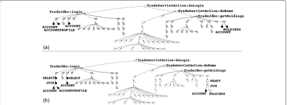
We will use this example to illustrate our initial work on code partitioning which, as highlighted above, led to improvements in performance as we moved parts of the code to the cloud and exploited its lower costs. Intuitively, by forcing certain data tables (account & accountprofile) to remain on premise, then code that manipulates these data elements is likely to remain on premise so that it stays close to the associated data and that communication times (and costs) do not become excessive. The diagram below, Figure 2(a), shows the call-tree of function execu-tion in the applicaexecu-tion-tier as well as data-tier query plans at the leaves. In the figure, we see three categories of com-ponents: (i) data on premise shown as black nodes, (ii) functions on premise as gray nodes, and (iii) functions in the cloud as white nodes.
As can be seen in Figure 2a, because, in our initial ap-proach, we are unable to partition data, we pin data to premise (account and holding) and so as expected, this forces significant amounts of code to stay on premise. However, as can also be seen from Figure 2a, some code can be moved to the cloud and our initial investigation (reported in section 3) explores what flexibility we had in this placement and the resulting performance and cost trade-offs.
In contrast, once we have the flexibility to address both code and data partitioning we have a more sophis-ticated tool available and so can explore moving data to the cloud, which obviously, will also have an affect on code placement. Figure 2b shows the output of our
cross-tier partitioning for doLogin. The figure shows the call-tree of function execution in the application-tier as well as data-tier query plans at the leaves. In the figure, we see four categories of components: (i) data on prem-ise shown as black nodes, (ii) a new category of data in the cloud as square nodes, (iii) functions on premise as gray nodes, and (iv) functions in the cloud as white nodes.
As can be seen, once we have the ability to partition data and move some of it, in Figure 2b Holdings, to the cloud, we are then able to move significantly more code to the cloud and so exploit its benefits. We explain the details of this in section 4.
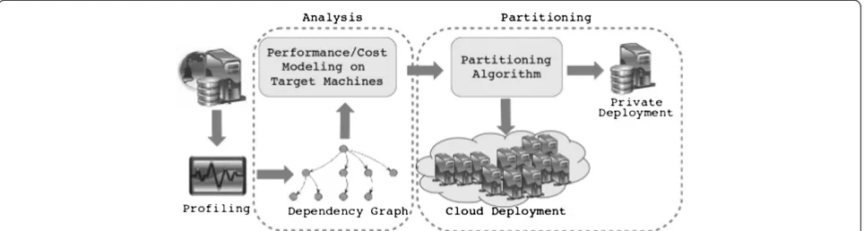
2.1 Overall methodology
To address application tier and data tier partitioning, we follow the methodology shown in Figure 3. The applica-tion is initially profiled by measuring execuapplica-tion time on a reference machine and collecting the data exchanges between software functions and data entities. Using this profile information, a dependency graph is developed which weaves application-tier and data-tier dependencies into a single cohesive dependency graph. The graph can then be analyzed to examine the effects of applying different cost models and placement constraints. Fi-nally, the dependency graph can be converted into an optimization problem that captures requirements both at the application-tier and data-tier and then solved using binary integer linear programming (BIP) to partition the application.
3 Application-tier partitioning
Our initial work focused on application-tier partitioning and attempted to exploit aspects of cloud infrastructure
in such a way as to improve the code partitioning algo-rithm. In particular, we wanted to understand if the asymmetric nature of cloud communication costs (i.e. in-bound data costs do not equal out-bound data costs), could be exploited to improve partitioning where one goal is to reduce overall execution costs of the application. To achieve this goal, we provide a new formulation of application partitioning as a binary integer programming optimization problem. This process consists of three high-level steps described above, (i) profiling, (ii) analysis, (iii) generating the BIP constraints and objective function.
3.1 Application profiling and analysis
Our process for application partitioning starts by taking an existing web application and applying in-strumentation to its binaries. The software is then exercised on representative workloads, using the in-strumentation to collect data on measured CPU usage and frequency of execution for software functions as well as data exchange between them. This work builds on our previous work where we explore online profiling of live execution in a cloud setting [9]. In that work, we showed how to provide low-overhead profiling of live application deployment using sampling. This allows profiles to account for popularity observed during usage by real customers. This log of profiling information will be converted to the relevant variables and costs of a BIP.
The log of profile data is converted to a graph model before being converted to a BIP, as shown in Figure 3. LetApp(V,E)represent a model of the application, where
forall v∈V,vcorresponds to a function execution in the application. Next,e(u,v)∈Eis a directed edge fromuto
vin the function call graph for the profiled application. Figure 2(a) and (b) show the visual graphical representa-tion of App(V,E) which is produced by our tool for visualization by software developers. For each v∈V we define exec(v) to represent the average profiled cost of
executing v on-premise and exec' (v) to represent the average profiled cost of executing v in the cloud. We also definelatency(u,v) to represent the latency cost on
e(u,v) and calculate the communication costcomm(u,v) fore(u,v) as follows:
comm uð ;vÞ ¼ latency uð ;vÞ þd uð ;vÞ commCost ð3:1Þ
WherecommCostis the cloud charges for each byte of data transfer, and d(u,v) represents the bytes of data exchange alonge(u,v).
3.2 BIP constraints and objective
Binary Integer Programming has been utilized previously for partitioning of applications (although not leveraging an asymmetric data exchange model or a cross-tier partitioning). A binary integer program consists of the following:
Binary variables: A set of binary variablesx1,, x2,…
xn∈{0,1}.
Constraints: A set of linear constraints between
variables where each constraint has the form: c1x1+ c2x2+…+ cnxn{≤,=,≥} cmwhere ciare all
constants
Objective: A linear expression to minimize or
maximize: cost1x1+ cost2x2+…+ costnxn, with each
costibeing the cost charged to the model when
xi= 1.
The job of a BIP optimizer is to choose the set of values for the binary variables which minimize/maximize this expression. For this purpose we convert our model of application profiling to a BIP and use an existing off-the-shelf BIP solver to optimize for placement of functions on either the public cloud or private premise.
For every nodeuin the dependency graph we consider a variable x(u) in the BIP formulation, where the set s
refers to entities placed on-premise and the set t refers to entities placed in the cloud.
x uð Þ∈f0;1g
∀x uð Þ∈s; x uð Þ ¼0
∀x uð Þ∈t; x tð Þ ¼1
ð3:2Þ
With all the above constraints, the following objective can then be defined:
minX
u∈V x uð Þ exec
0
u
ð Þ þð1−x uð ÞÞ exec uð Þ
ð Þ
þX
u;v
ð Þ∈Eðx uð Þ−x vð ÞÞ
2
comm uð ;vÞ
ð3:3Þ
where the quadratic expression in the objective func-tion can be relaxed by making the expansion suggested in [10].
∀ðu;vÞ∈E e uð ;vÞ≥0; e uð ;vÞ≤1
∀ðu;vÞ∈E e0ðu;vÞ≥0; e0ðu;vÞ≤1
∀ðu;vÞ∈E x uð Þ−x vð Þ þe uð ;vÞ≥0
∀ðu;vÞ∈E x vð Þ−x uð Þ þe0ðu;vÞ≥0
ð3:4Þ
This expansion introduces auxiliary variables e'(u,v) for each edge in the original model; these new variables are used for emulating the constraints of a quadratic function by a combination of linear functions and don’t directly map to the system being modeled. Their inter-pretation is described further below. Now the objective function of Equation 3.3 is converted to the following formulation. We refer to the objective of Equation 3.5 as
Symmetric IPas it does not distinguish between inbound and outbound communication costs:
minX
u∈V x uð Þ exec
0
u
ð Þ þð1−x uð ÞÞ exec uð Þ
ð Þ
þX
u;v
ð Þ∈E e uð ;vÞ þe
0ðu;vÞ
ð Þ commðu;vÞ
ð3:5Þ
Interpreting this equation, e(u,v) and e' (u,v) will be 0 if both x(u) and x(v) are assigned to the same host but e(u,v) will be 0 and e'(u,v) will be 1 if x(u) is assigned to t and x(v) is assigned to s. Otherwise
e(u,v) will be 1 and e' (u,v) will be 0 if x(u) is on s
and x(v) is on t. An immediate benefit of being able to determine module placements in relation to one another is the ability to formulate the asymmetric data exchange charges for a cloud deployment into the partitioning problem. Benefiting from the expansion in Equation 3.4, we can add public cloud’s asymmetric
billing charges to the communication cost of Equation 3.1 as follows:
comm0ðu;vÞ ¼ðe uð ;vÞ þe0ðu;vÞÞ latency uð ;vÞ þasync uð ;vÞ cloudCommCost e0ðu;vÞ þasync vð ;uÞ
premiseCommCost e uð ;vÞ ð3:6Þ whereasync(u,v) stands for quantity of data transfer from cloud to the premise withx(u) being in the cloud andx(v) being on-premise, and async(v,u) represents quantity of data transfer from premise to the cloud wherex(u) is on-premise and x(v) is in the cloud. We also calculate the monetary cost for latency(u,v) based on the formulation provided in our previous work which allows the tool user to tune the cost to match the specific deployment situ-ation. Essentially the user just provides a weighted param-eter to penalize optimization solutions which increase the average request latency, further details are described in [5]. The above formulation, combined with separation of outgoing and ingoing data to a function during application profiling leads to a more accurate cost optimization of the target software service for a hybrid deployment. Following the changes above, the objective function of Equation3.5
can be updated by replacing (e(u,v) +e' (u,v)) ×comm(u,v) withcomm' (u,v). In our evaluations, we refer to this new IP formulation as theAsymmetric IP.
As a concrete example of how the asymmetric algorithm works within the context of DayTrader, we provide an ex-ample in Figure 4 of part of the code partitioning suggested by the asymmetric algorithm when applied to DayTrader’ -sApp(V,E). Figure 4 shows a piece for the request type
doAccount. Assuming that theaccountprofiledatabase table is constrained to stay on-premise, in a symmetric partition-ing algorithm separatpartition-ing getAccountDatafrom doAccount
(7 ~ KB of data exchange) is preferred over cutting execute-Query(13 ~ KB of data exchange). In an asymmetric parti-tioning however, the algorithm will assign no costs to the edges going to the cloud. For this reason, cutting execute-Query to be pushed to the premise has equivalent cost overhead (1 ~ KB) compared to cutting getAccountData. However, there is a gain in cuttingexecuteQueryin that by pushing only this method to the premise, all other function nodes (black nodes) can be placed in the cloud, benefiting from more scalable and cheaper resources.
3.3 Asymmetric vs. symmetric partitioning
We used the following setup for the evaluation: for the premise machines, we used two 3.5 GHz dual core machines with 8.0 GB of memory, one as the application server and another as our database server. Both ma-chines were located at our lab in Vancouver, and were connected through a 100 Mb/sec data link. For the cloud machines, we used an extra large EC2 instance with 8 EC2 Compute Units and 7.0 GB of memory as our application server and another extra large instance as our database server. Both machines were leased from Amazon’s US West region (Oregon) and were con-nected by a 1 Gb/sec data link. We use Jetty as the Web server and Oracle 11 g Express Edition as the database servers. We measured the round-trip latency between the cloud and our lab to be 15 milliseconds. Our intention for choosing these setups is to create an environment where the cloud offers the faster and more scalable environ-ment. To generate load for the deployments, we launched simulated clients from a 3.0 GHz quad core machine with 8 GB of memory located in our lab in Vancouver.
Figures 5 and 6 show the results of data exchange for symmetric versus asymmetric partitioning algorithms. From the data, we can see two main results. First, considering each bar as a whole (ignoring the breakdown of each bar into its two components) and comparing the same request between the two figures (e.g. doLogin, Figure 5 vs. doLogin, Figure 6), we can notice the difference of aggregate data exchange for the two approaches. Here we see that in some cases, the aggregate data exchange is greater for the symmetric approach but in other cases it is greater for the asymmetric approach. However, there is a clear trend for asymmetric to be greater. On average over all the requests, asymmetric partitioning increases the overall amount of
data going from the premise to the cloud by a factor of 82%. However, when we breakdown the aggregate data exchange into two components (ingoing and outgoing), we can see an advantage of the asymmetric approach.
This second result of Figures 5 and 6 can be seen by comparing the ratio of ingoing and outgoing data for each request type. Here we see the asymmetric algorithm re-duces the overall amount of data going from the cloud to the premise (red part of the chart). This can be a major fac-tor when charges associated with data going from the cloud to the premise are more expensive than charges for data going from the premise to the cloud. On average over the request types, asymmetric partitioning reduces the overall amount of data going from the cloud to the premise by a factor of 52%. As we see in the next experiment, this can play a role in decreasing the total cost of deployment.
Figures 7 and 8 show the overall average request pro-cessing time for each request type when using symmetric compared to asymmetric partitioning. Each bar is broken down into two components: average time spent processing the request in the cloud and average time spent processing the request on premise. Again we see two results, that somewhat mirror the two results from Figures 5 and 6. First, again considering each bar as a whole, the total re-quest processing time in each case is similar. In some Figure 4A high-level model of how different partitioning
algorithms would choose the placement of code and data components between the public and the private cloud.For each of the three lines, code elements and database tables falling below the line are considered to be placed on premise and all the other elements are placed in the public cloud.
Figure 5Average profiled data transfer for request types in DayTrader using the Symmetric IP.
cases, the total processing time is greater for the symmet-ric approach but in other cases it is greater for the asym-metric approach. However, the asymasym-metric partitioning allows for more of the code to be moved to the cloud (with its associated cheaper resources for deployment costs) and so the overall cost of execution is also reduced.
This second result of Figures 7 and 8 can be seen by comparing ratio of cloud processing time and premise processing time for each request. We see that asymmetric partitioning increases the overall usage of cloud resources. Overall, asymmetric partitioning moves an additional 49% of execution time for an application to the cloud. With cloud resources being the cheaper resources, this will translate to cost savings for charges associated to CPU resources.
From the results of these experiments, we saw the sig-nificant effect that asymmetric partitioning had in enabling more code to be pushed to the cloud by the optimizer. This is because costs of data transfer to the code running on the public cloud are less expensive than data coming from the public cloud. However, while closely examining the resulting partitioning in our visualization we noticed a common case where some code was rarely ever pushed to the public cloud, making automated partitioning less effective. This case always occurred for code which was tightly coupled to some persistent data which we assumed was always stored on premise. This phenomenon is
illustrated well by the function nodes in Figure 2(a) which are rooted at the function TradeJdbc:getHoldings. Based on this observation we were motivated to investigate the potential of extending our approach to scenarios where persistent data could be distributed across both the public cloud and private premise. Next in Section 5, we augment the asymmetric code partitioning approach with this cross-tier, code and data partitioning.
4 Data-tier partitioning
The technical details of extending application-tier parti-tioning to integrate the data-tier are motivated by four re-quirements: (i) weighing the benefits of distributing queries, (ii) comparing the trade-offs between join orders, (iii) taking into account intra-request data-dependencies and (iv) providing a query execution model comparable to application-tier function execution. In this section, we first further motivate cross-tier partitioning by describing each of these points, then we cover the technical details for the steps of partitioning as they relate to the data-tier. Data in our system can be partitioned at the granularity of tables. We choose this granularity for two reasons: (i) it allows us to transparently partition applications using a lightweight middleware on top of an existing distributed database (we used Oracle in our experiments), (ii) tables are already a natural unit of security isolation for existing RDBMS con-trols. Transparently partitioning row-level or column-level Figure 7Average profiled execution times for request types in DayTrader using the Symmetric IP.
data would not be difficult from the perspective of our BIP model, but it would require additional sophistication in our middleware or a special-purpose database. We focus on a data-tier implemented with a traditional SQL database. While some web application workloads can benefit from the use of alternative NoSQL techniques, we chose to focus initially on SQL due to its generality and widespread adoption.
First, as described in Section 2, placing more of the less-sensitive data in the cloud will allow for the corre-sponding code from the application-tier to also be placed in the cloud, thus increasing the overall efficiency of the deployment and reducing data transfer. However, this can result in splitting the set of tables used in a query across public and private locations. For our DayTrader example, each user can have many stocks in her holding which makes the holding table quite large. As shown in Figure 2, splitting the join operation can push the holdings table to the cloud (square nodes) and eliminate the traffic of moving its data to the cloud. This splitting also maintains our con-straint to have the privacy sensitive account table on the private premise. An effective modeling of the data-tier needs to help the BIP optimizer reason about the trade-offs of distributing such queries across the hybrid architecture.
Second, the order that tables are joined can have an ef-fect not only on traditional processing time but also on round-trip latency. We use a running example throughout this section of the query shown in Figure 9, with two dif-ferent join orders, left and right. If the query results are processed in the public cloud where the holding table is in the cloud and account and accountprofile are stored on the private premise, then the plan on the left will incur two-round trips from the public to private locations for distributed processing. On the other hand, the query on the right only requires one round-trip. Modeling the data-tier should help the BIP optimizer reason about the cost of execution plans for different placements of tables.
Third, some application requests execute more than one query. In these cases, it may be beneficial to partition functions to group execution with data at a single location. Such grouping helps to eliminate latency overhead otherwise needed to move data to the location where the application-tier code executes. An example of this is
shown in Figure 2(b), where a sub-tree of function exe-cutions for TradeJdbc:loginis labeled as “private” (gray nodes). By pushing this sub-tree to the private premise, the computation needed for working over account and
accountprofiledata in the two queries underTradeJdbc: logincan be completed at the premise without multiple round-trips between locations.
Fourth, since the trade-offs on function placement depend on the placement of data and vice-versa, we need a model that can reason simultaneously about both application-tier function execution and query plan execution. Thus the model for the data-tier should be compatible for integration with an approach to application partitioning such as the one described in Section 3.
4.1 Database profiling with explain plan
Having motivated the need for a model of query execu-tion to incorporate the data-tier in a cross-tier partiexecu-tion- partition-ing, we now explore the details. Figure 10 shows an extended version of Figure 3 in which we have broken out the code and data parts of the 3 phase process, (i) profiling, (ii) analysis, (iii) generating the BIP constraints and objective function. For data, the overall process is as follows. We first profile query execution using Explain Plan. This information is used to collect statistics for query plan operators by interrogating the database for different join orders (Section 4.2). The statistics are then used to generate both BIP constraints (Section 4.3) and a BIP objective function (Section 4.4). Finally, these con-straints and objective are combined with that from the application-tier to encode a cross-tier partitioning model for a BIP solver.
Profiling information is available for query execution through the Explain Plan SQL command. Given a par-ticular query, this command provides a tree- structured result set detailing the execution of the query. We use a custom JDBC driver wrapper to collect information on the execution of queries. During application profiling (cf. Section 3) whenever a query is issued by the application-tier, our JDBC wrapper intercepts the query and collects the plan for its execution. The plan returned by the database contains the following information:
1. type(op): Each node in the query plan is an operator such as a join, table access, selection (i.e. filter), sort, etc. To simplify presentation of the technical details, we assume that each operator is either a join or a table access. Other operators are handled by our
implementation but they don’t add extra complexity
compared to a join operator. For example, in Figure9,
the selection (i.e. filter) operators are elided. We leverage
the database’s own cost model directly by recording
from the provided plan how much each operator costs.
Hence, we don’t need to evaluate different operator
implementations to evaluate their costs. On the other hand, we do need to handle joins specially because table placement is greatly affected by their ordering. 2. cpu(op): This statistic gives the expected time of
execution for a specific operator. In general, we assume that the execution of a request in a hybrid web application will be dominated by the CPU processing of the application- tier and the network latency. So in many cases, this statistic is negligible. However, we include it to detect the odd case of expensive query operations which can benefit from executing on the public cloud.
3. size(op): This statistic captures the expected number of bytes output by an operator which is equal to the expected number of rows times the size of each retrieved row. From the perspective of the plan tree-structure, this is the data which flows from a child operator to its parent.
4. predicates(joinOp): Each join operator combines two inputs based on a set of predicates which relate those inputs. We use these predicates to determine if alternative join orders are possible for a query. When profiling the application, the profiler observes and collects execution statistics only for plans that get executed but not for alternative join orders. However, the optimal plan executed by the database engine in a distributed hybrid deployment can be different from the one observed during profiling. In
order to make the BIP partitioner aware of alternative orders, we have extended our JDBC wrapper to consult the database engine and examine the alternatives by utilizing a combination of Explain Plan and join order hints. Our motivation is to leverage the already existing cost model from a production database for cost estimation of local operator processing, while still covering the space of all query plans. The profiler also captures which sets of tables are accessed together as part of an atomic transaction. This information is used to model additional costs of applying a two-phase commit protocol, should the tables get partitioned.
4.2 Join order enumeration
We need to encode enough information in the BIP so it can reason over all possible plans. Otherwise, the BIP optimizer would mistakenly assume that the plan executed during our initial profiling is the only one possible. For ex-ample, during initial profiling on a single host, we may only observe the left plan from Figure 5. However, in the ex-ample scenario, we saw that the right plan introduces fewer round-trips across a hybrid architecture. We need to make sure the right plan is accounted for when deciding about table placement. Our strategy to collect the necessary infor-mation for all plans consists of two steps: (i) gather statistics for all operators in all plans irrespective of how they are joined, and (ii) encode BIP constraints about how the oper-ators from step (i) can be joined. Here we describe step 1 and then describe step 2 in the next subsection. The novelty of our approach is that instead of optimizing to a specific join order in isolation of the structure of application-tier execution, we encode the possible orders together with the BIP of the application-tier as a combined BIP.
(the“outer relation”). The identity of the inner relation and the set of tables comprising the outer relation uniquely de-termine the estimated best cost for an individual join oper-ator. This is true regardless of the in which the outer relation was derived [11]. For convenience in our presenta-tion, we call this information the operator’s id, because we use it to represent an operator in the BIP. For example, the root operator in Figure 9a takesaccountProfileas an inner input and{holding, account}as an outer input. The opera-tor’s id is then{(holding, account), accountProfile}. We will refer to the union of these two inputs as a join set (the set of tables joined by that operator). For example, the join set of the aforementioned operator is {holding, account, accountProfile}. Notably, while the join sets for the roots of Figure 9a & b are the same, Figure 9b’s root node has the operator id{(accountProfile, account), holding} allow-ing us to differentiate the operators in our BIP formula-tion. Our task in this section is to collect statistics for the possible join operators with unique ids.
Most databases provide the capability for developers to provide hints to the query optimizer in order to force certain joins. For example in Oracle, a developer can use the hint LEADING(X, Y, Z, …). This tells the optimizer to create a plan whereXandYare joined first, then their intermediate result is joined with Z, etc. We use this capability to extract statistics for all join orders.
Algorithm 1 takes as input a query observed during pro-filing. In line 2, we extract the set of all tables referenced in the query. Next, we start collecting operator statistics for joins over two tables and progressively expand the size through each iteration of the loop on line 3. The table t, selected for each iteration of line 4 can be considered as the inner input of a join. Then, on line 5 we loop through all sets of tables of sizeiwhich don’t containt. On line 6, we verify iftis joinable with the setSby making sure that at least one table in the setSshares a join (access) predi-cate with t. This set forms the outer input to a join. Fi-nally, on line 7, we collect statistics for this join operator by forcing the database to explain a plan in which the join order is prefixed by the outer input set, followed by the inner input relation. We record the information for each operator by associating it with its id. For example, con-sider Figure 4 as the inputQto Algorithm 1.
In a particular iteration of line 5, i might be chosen as 2 and t as accountProfile. Since account-Profile has a predicate shared with account, S could be chosen as the set of size 2: {account, holdings}. Now on line 6, explainPlanWithLeadingTables({ac-count, holdings}, accountProfile) will get called and the statistics for the join operator with the corresponding id will get recorded.
The bottom-up structure of the algorithm follows similarly to the classic dynamic programming algo-rithm for query optimization [11]. However, in our case we make calls into the database to extract costs by leveraging Explain Plan and the LEADING hint. The complexity of Algorithm 1 is O(2n) (where n is the number of tables); which is the same as the clas-sic algorithm for query optimization [11], so our ap-proach scales in a similar fashion. Even though this is exponential, OLTP queries typically don’t operate on over more than ten tables.
4.3 BIP constraints
Now that we know the statistics for all operators with a unique id, we need to instruct the BIP how they can be composed. Our general strategy is to model each query plan operator,op, as a binary vari-able in a BIP. The varivari-able will take on the value 1 if the operator is part of the query plan which min-imizes the objective of the BIP and 0 otherwise. Each possible join set is also modeled as a variable. Constraints are used to create a connection between operators that create a join set and operators that consume a join set (cf. Table 1). The optimizer will choose a plan having the least cost given both the optimizer’s choice of table placement and function execution placement (for the application-tier). Each operator also has associated variables opcloudand
oppremisewhich indicate the placement of the
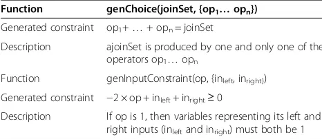
Our algorithm to formulate these composition con-straints makes use of two helper functions as shown in Table 1, namely genChoice and genInputConstraint. When these functions are called by our algorithms, they append the generated constraint to the BIP that was already built for the application-tier. The first function, genChoice, encodes that a particular join set may be derived by multiple possible join operators (e.g., {holding, account, accountprofile} could be de-rived by either of the root nodes in Figure 9). The second function, genInputConstraint, encodes that a particular join operator takes as inputs the join sets of its two children. It ensures that if op is selected, both its children’s join sets (inleft and inright)are se-lected as well, constraining which subtrees of the execution plan can appear under this operator. The
“≥” inequality in Table 1 helps to encode the boolean logic op→inleft ⋀ inright.
Starting with the final output join set of a query, Algorithm 2 recursively generates these constraints encoding choices between join operators and how parent operators are connected to their children. It starts on line 2 by calling a function to retrieve all operator ids which could produce that join set (these operators were all collected during the execution of Algorithm 1). It passes this information to genChoice
on line 3. On line 4, we loop over all these operator ids, decomposing each into its two inputs on line 5. This information is then passed to genInputCon-straint. Finally on line 7, we test for the base case of
a table access operator. If we have not hit the base case, then the left input becomes the join set for recursion on line 8.
4.4 BIP objective
Creating the optimization objective function consists of two parts: (i) determining the costs associated with the execution of individual operators, and (ii) creating a mathematical formulation of those costs. The magnitude of the execution cost for each oper-ator and the communication cost between operoper-ators that are split across the network are computed using a similar cost model to previous work [12]. This ac-counts for the variation between local execution and distributed execution in that the latter will make use of a semi-join optimization to reduce costs (i.e. in-put data to a distributed join operator will transmit only the columns needed to collect matching rows). We extend the previous cost model to account for possible transaction delays. We assume that if the tables involved in an atomic transaction are split across the cloud and the private premise, by default the transaction will be resolved using the two-phase commit protocol.
Performance overhead from atomic two-phase distrib-uted transactions comes primarily from two sources: protocol overhead and lock contention. Protocol over-head is caused by the latency of prepare and commit messages in a database’s two-phase commit protocol. Lock contention is caused by queuing delay which in-creases as transactions over common table rows become blocked. We provide two alternatives to account for such overhead:
– For some transactions, lock contention is negligible.
This is because the application semantics don’t
induce sharing of table rows between multiple user sessions. For example, in DayTrader, although
Table 1 Constraint generation functions
Function genChoice(joinSet, {op1…opn})
Generated constraint op1+…+ opn= joinSet
Description ajoinSet is produced by one and only one of the operators op1…opn
Function genInputConstraint(op, {inleft, inright})
Generated constraint −2 × op + inleft+ inright≥0
Description If op is 1, then variables representing its left and right inputs (inleftand inright) must both be 1
Table 2 Functions for generating objective helper constraints
Function genAtMostOneLocation(op)
Generated constraint opcloud+ oppremise=op
Description If the variable representingopis 1, then either the variable representing it being placed in the cloud is 1 or the variable representing it being place in the premise is 1
Function genSeparated(op1,op2)
Generated constraint op1, cloud+ op2, premise-cutop1, op2≤1
op1, premise+ op2, cloud-cutop1, op2≤1 Description If the variables representing the locations of
two operators are different, then the variable
Account and Holdings tables are involved in an atomic transaction, specific rows of these tables are only ever accessed by a single user
concurrently. In such cases we charge the cost of two extra round-trips between the cloud and the private premise to the objective function, one to prepare the remote site for the transaction and another to commit it.
– For cases where lock contention is expected to be
considerable, developers can request that certain tables be co-located in any partitioning suggested by our tool. This prevents locking for transactions over those tables to be delayed by network latency. Since such decisions require knowledge of application semantics that are difficult to infer automatically, our tool provides an interactive visualization of partitioning results, as shown in
Figure 2(a) and (b). This allows developers to
work through different “what-if” scenarios of
table co-location constraints and the resulting suggested partitioning.
Next, we need to encode information on CPU and data transmission costs into the objective function. In addition to generating a BIP objective, we will need
some additional constraints that ensure the calculated objective is actually feasible. Table 2 shows functions to generate these constraints. The first constraint spe-cifies that if an operator is included as part of a chosen query plan (its associated id variable is set to 1), then either the auxiliary variable opcloud or oppremise will have to be 1 but not both. This enforces a single place-ment location for op. The second builds on the first and toggles the auxiliary variable cutop1,op2 when
op1cloud and op2premise are 1, or when op1premise and
op2cloudare 1.
The objective function itself is generated using two functions in Table 3. The first possibly charges to the objective function either the execution cost of the oper-ator on the cloud infrastructure or on the premise infra-structure. Note that it will never charge both due to the constraints of Table 2. The second function charges the communication cost between two operators if the asso-ciated cut variable was set to 1. In the case that there is no communication between two operators this cost is simply 0.
Algorithm 3 takes a join set as input and follows a similar structure to Algorithm 2. The outer loop on line 3, iterates over each operator that could produce the particular join set.
Table 3 Functions for generating objective function
Function genExecutionCost(op)
Generated objective component opcloud× execCostcloud(op) +oppremise× execCostpremise(op)
Description If the variable representingopdeployed in the cloud/premise is 1, then charge the associated cost of executing it in the cloud/premise respectively
Function genCommCost(op1,op2)
Generated objective component cutop1, op2× commCost(op1,op2)
It generates the location constraints on line 4 and the execution cost component to the objective function on line 5. Next, on line 7, it iterates over the two inputs to the operator. For each, it extracts the operators that could produce that input (line 8) and generates the communica-tion constraint and objective funccommunica-tion component. Finally, if the left input is not a base relation (line 11), it recurses using the left input now as the next join set.
Having appended the constraints and objective compo-nents associated with query execution to the application-tier BIP, we make a connection between the two by encoding the dependency between each function that executes a query and the possible root operators for the associated query plan.
5 Implementation
We have implemented our cross-tier partitioning as a framework. It conducts profiling, partitioning, and distri-bution of web applications which have their business logic implemented in Java. Besides the profiling data, the analyzer also accepts a declarative XML policy and cost parameters. The cost parameters encode the monetary costs charged by a chosen cloud infrastructure provider and expected environmental parameters such as available bandwidth and network latency. The declarative policy al-lows for specification of database table placement and co-location constraints. In general we consider the placement of privacy sensitive data to be the primary consideration for partitioning decisions. However, developers may wish to monitor and constrain the placement of function execu-tions that operate over this sensitive data. For this purpose we rely on existing work using taint tracking [13] which we have integrated into our profiler.
For partitioning, we use the off-the-shelf integer pro-gramming solverlp_solve[14] to solve the discussed BIP optimization problem. The results lead to generating a distribution plan describing which entities need to be separated from one another (cut-points). A cut-point may separate functions from one an- other, functions from data, and data from one another. Separation of code and data is achievable by accessing the database engine through the database driver. Separating inter-code or inter-data dependencies requires extra middleware.
For functions, we have developed a bytecode rewriting engine as well as an HTTP based remote call library that takes the partitioning plan generated by the analyzer, injects remote call code at each cut-point, and serializes data between the two locations. This remote call instru-mentation is essentially a simplified version of J-Orchestra [15] implemented over HTTP (but is not yet as complete as the original J-Orchestra work). In order to allow for distribution of data entities, we have taken advantage of Oracle’s distributed database management system (DDBMS). This allows for tables remote to a local Oracle
DBMS, to be identified and queried for data through the local Oracle DBMS. This is possible by providing a database link (@dblink) between the local and the remote DBMS systems. Once a bidirectional dblink is established, the two databases can execute SQL state-ments targeting tables from one another. This allows us to use the distribution plan from our analyzer system to perform vertical sharding at the level of database tables. Note that the distributed query engine acts on the deploy-ment of a system after a decision about the placedeploy-ment of tables has been made by our partitioning algorithm. We have provided an Eclipse plugin implementation of the analyzer framework available online [16].
6 Evaluation
Now we evaluate our complete cross-tier partitioning on two different applications: DayTrader [8] (cf. Section 2) and RUBiS [17]. RUBiS implements the functionality of an auctioning Web site. Both applications have already been used in evaluating previous cloud computing re-search [17,18]. We can have 9 possible deployment variations with each of the data-tier and the application tier being (i) on the private premise, (ii) on the public cloud, or (iii) partitioned for hybrid deployment. Out of all the placements we eliminate the 3 that place all data in the cloud as it contradicts the constraints to have privacy sensitive information on-premise. Also, we consider deployments with only data partitioned as a subset of deployments with both code and data partitioned, and thus do not provide separate deployments for them. The remaining four models deployed for evaluations were as follows: (i) both code and data are deployed to the premise (Private-Premise); (ii) data is on-premise and code is in the cloud (Naive-Hybrid); (iii) data is on-premise and code is partitioned (Split-Code); and (iv) both data and code are partitioned (Cross-Tier).
For both DayTrader and RUBiS, we consider privacy incentives to be the reason behind constraining placement for some database tables. As such, when partitioning data, we constrain tables storing user information (accountand
accountprofile for DayTrader and users for RUBiS) to be placed on-premise. The remaining tables are allowed to be flexibly placed on-premise or in the cloud.
The details of machine and network setup are the same as described in Section 3.3, so we don’t repeat them here. In the rest of this section we provide the following evaluation results for the four deployments described above: execution times (Section 6.1), expected monetary deployment costs (Section 6.2), and scalability under vary-ing load (Section 6.3).
6.1 Evaluation of performance
of 100 requests per second, for ten minutes. By execu-tion time we mean the elapsed wall clock time from the beginning to the end of each servlet execution. Figure 11 shows those with largest average execution times. We model a situation where CPU resources are not under significant load. As shown in Figure 11, execution time in cross-tier partitioning is significantly better than any other model of hybrid deployment and is closely comparable to a non-distributed private premise deploy-ment. As an example, execution time for DayTrader’s doLogin under Cross-Tier deployment is 50% faster than Naıve-Hybrid while doLogin’s time for Cross-Tier is only 5% slower compared to Private-Premise (i.e., the lowest bar in the graph). It can also be seen that, for doLogin, Cross-Tier has 25% better execution time compared to Split-Code, showing the effectiveness of cross-tier partitioning compared to partitioning only at the application-tier.
Similarly for other business logic functionality, we note that cross-tier partitioning achieves considerable per-formance improvements when compared to other dis-tributed deployment models. It results in performance measures broadly similar to a full premise deployment. For the case of DayTrader - across all business logic functionality of Figure 11a - Cross-Tier results in an overall performance improvement of 56% compared to
Naive-Hybrid and a performance improvement of around 45% compared to Split-Code. We observed similar per-formance improvements for RUBiS. Cross-Tier RUBiS performs 28.3% better - across all business logic function-ality of Figure 11b - compared to its Naive-Hybrid, and 15.2% better compared to Split-Code. Based on the re-sults, cross-tier partitioning provides more flexibility for moving function execution to the cloud and can signifi-cantly increase performance for a hybrid deployment of an application.
6.2 Evaluation of deployment costs
For computing monetary costs of deployments, we use parameters taken from the advertised Amazon EC2 service where the cost of an extra large EC2 instance is $0.48/hour and the cost of data transfer is $0.12/GB. To evaluate deployment costs, we apply these machine and data transfer costs to the performance results from Section 6.1, scale the ten minute deployment times to one month, and gradually change the ratio of premise-to-cloud deployment costs to assess the effects of varying cost of private premise on the overall deployment costs. As these input parameters are changed, we re-run the new inputs through our tool, deploy the generated source code partitions from the tool as separate Java
“war”archives, and run each experiment.
As shown in both graphs, a Private-Premise deploy-ment of web applications results in rapid cost increases, rendering such deployments inefficient. In contrast, all partitioned deployments of the applications result in more optimal deployments with Cross-Tier being the most efficient. For a cloud cost 80% cheaper than the private-premise cost (5 times ratio), DayTrader’s Cross-Tier is 20.4% cheaper than Private-Premise and 11.8% cheaper than Naive-Hybrid and Split-Code deployments. RUBiS achieves even better cost savings with Cross-Tier being 54% cheaper than Private-Premise and 29% cheaper than Naive-Hybrid and Split-Code. As shown in Figure 12a, in cases where only code is partitioned, a gradual increase in costs for machines on-premise eventually results in the algorithm pushing more code to the cloud to the point where all code is in the cloud and all data is on-premise. In such a situation Split-Code eventually converges to Naive-Hybrid; i.e., pushing all the code to the cloud. Similarly, Cross-Tier will finally stabilize. However since in Cross-Tier part of the data is also moved to the cloud, the overall cost is lower than Naive-Hybrid and Split-Code.
6.3 Evaluation of scalability
We also performed scalability analyses for both DayTrader and RUBiS to see how different placement choices affect application throughput. DayTrader comes with a random client workload generator that dispatches requests to all
available functionality on DayTrader. On the other hand, RUBiS has a client simulator designed to operate either in the browsing mode or the buy mode.
For both DayTrader and RUBiS we used a range of 10 to 1000 client threads to send requests to the applications in 5 minute intervals with 1 minute ramp-up. For RUBiS, we used the client in buy mode. Results are shown in Figure 13. As the figure shows, for both applications, after the number of requests reaches a certain threshold, Private-Premise becomes overloaded. For Naive-Hybrid and Split-Code, the applications progressively provide better throughput. However, due to the significant bottle-neck when accessing the data, both deployments maintain a consistent but rather low throughput during their execu-tions. Finally, Cross-Tier achieved the best scalability. With a big portion of the data in the cloud, the underlying resources for both code and data can scale to reach a much better overall throughput for the applications. Despite having part of the data on the private premise, due to its small size the database machine on premise gets congested at a slower rate and the deployment can keep a high throughput.
7 Related work
Our research bridges the two areas of application and database partitioning but differs from previous work in that it uses a new BIP formulation that considers both areas. Our focus is not on providing all of the many
features provided by every previous project either on application partitioning or database partitioning. In-stead, we have focused on providing a new interface between the two using our combined BIP. We describe the differences in more detail by first describing some related work in application partitioning and then data-base partitioning.
Application Partitioning:Coign [19] is an example of
classic application partitioning research which provides partitioning of Microsoft COM components. Other work focuses specifically on partitioning of web/mobile ap-plications such as Swift [20], Hilda [21], and AlfredO [22]. However that work is focused on partitioning the application-tier in order to off-load computation from the server-side to a client. That work does not handle partitioning of the data-tier.
Minimizing cost and improving performance for de-ployment of software services has also been the focus of cloud computing research [23]. While approaches like Volley [24] reduce network traffic by relocating data, others like CloneCloud [2], CloudwardBound[3], and our own Manticore [5] improve performance through relocation of server components. Even though Volley examines data dependencies and CloneCloud, Cloudward Bound, and Manticore examine component or code dependencies, none of these approaches combine code and data dependencies to drive their partitioning and distribution decisions. In this paper, we demonstrated
how combining code and data dependencies can provide a richer model that better supports cross-tier partitioning for web application in a hybrid architecture.
Database Partitioning:Database partitioning is
gener-ally divided into horizontal partitioning and vertical parti-tioning [25]. In horizontal partiparti-tioning, the rows of some tables are split across multiple hosts. A common motiv-ation is for load-balancing the database workload across multiple database manager instances [26,27]. In vertical partitioning, some columns of the database are split into groups which are commonly accessed together, improving access locality [9]. Unlike traditional horizontal or vertical partitioning, our partitioning of data works at the granu-larity of entire tables. This is because our motivation is not only performance based but is motivated by policies on the management of data resources in the hybrid archi-tecture. The granularity of logical tables aligns more nat-urally than columns with common business policies and access controls. That being said, we believe if motivated by the right use-case, our technical approach could likely be extended for column-level partitioning as well.
8 Limitations, future work, and conclusion
on partitioning. After partitioning, a developer may also want to consider changes to the implementation to handle some transactions in an alternative fashion, e.g. providing forward compensation. Also as noted, our current imple-mentation and experience is limited to Java-based web ap-plications and SQL-based databases.
In future work we plan to support a more loosely coupled service-oriented architecture for partitioning applications. Our current implementation of data-tier partitioning relies on leveraging the distributed query engine from a production database. In some environ-ments, relying on a homogeneous integration of data by the underlying platform may not be realistic. We are currently working to automatically generate REST inter-faces to integrate data between the public cloud and private premise rather than relying on a SQL layer.
In this paper we have demonstrated that combining code and data dependency models can lead to cheaper and better performing hybrid deployment of Web applica-tions. Our initial approach considered only code partition-ing but different from previous approaches it was sensitive to the ingress or egress flow of data to/from the public cloud. Our initial evaluation showed this to be promising but still limited since placement of data was fixed at the private premise. By extending this approach to cross-tier partitioning we demonstrated further improvement. In particular, our evaluation showed that for our evaluated applications, combined code and data partitioning can achieve up to 56% performance improvement compared to a naıve partitioning of code and data between the cloud and the premise and a more than 40% performance im-provement compared to when only code is partitioned (see Section 6.1). Similarly, for deployment costs, we showed that combining code and data can provide up to 54% expected cost savings compared to a fully premise de-ployment and almost 30% expected savings compared to a naively partitioned deployment of code and data or a de-ployment where only code is partitioned (cf. Section 6.2).
Competing interests
The authors declare that they have no competing interests.
Authors’contributions
NK participated in the study design and carried out the experimental work on both application and data tier partitioning, developed the experimental setup and gathered all data from the experiments. EW helped formulate the original study design, participated in the design of the approach to both application and data tier partitioning and analysis of both data sets. RL helped formulated the original study design, participated in the design of the asymmetric/symmetric approach and in the analysis of the both data sets. All authors participated in writing the manuscript and final approval.
Received: 22 July 2014 Accepted: 17 November 2014
References
1. Armbrust A, Fox A, Griffith R, Joseph AD, Katz RH, Konwinski A, Lee G, Patterson DA, Rabkin A, Stoica I, Zaharia M (2009) Above the Clouds: A Berkeley View of Cloud Computing., Technical Report UCB/EECS-2009-28, UC Berkeley
2. Chun BG, Ihm S, Maniatis P, Naik M, Patti A (2011) Clonecloud: Elastic Execution Between Mobile Device and Cloud, Proceeding of EuroSys., p 301, doi:10.1145/1966445.1966473
3. Hajjat M, Sun X, Sung YWE, Maltz D, Rao S, Sripanidkulchai K, Tawarmalani M (2010) Cloudward Bound: Planning for Beneficial Migration of Enterprise Applications to the Cloud. In: Proc. of SIGCOMM., p 243, doi:10.1145/ 1851275.1851212
4. Leymann F, Fehling C, Mietzner R, Nowak A, Dustdar S (2011) Moving applications to the cloud: an approach based on application model enrichment. J Cooperative Information Systems 20(3):307–356 5. Kaviani N, Wohlstadter E, Lea R (2012) Manticore: A Framework for
Partitioning of Software Services for Hybrid Cloud, Proceedings of IEEE CloudCom., p 333, doi:10.1109/CloudCom.2012.6427541
6. Khadilkar V, Kantarcioglu M, Thuraisingham B (2011) Risk-Aware Data Processing in Hybrid Clouds, Technical report, University of Texas at Dallas 7. Schrijver A (1998) Theory of Linear and Integer Programming. Wiley & Sons,
Hoboken, NJ
8. DayTrader 3.0.0. http://svn.apache.org/repos/asf/geronimo/daytrader/tags/ daytrader-parent-3.0.0/. Accessed 23 Jun 2014.
9. Kaviani N, Wohlstadter E, Lea R (2011) Profiling-as-a-Service: Adaptive Scalable Resource Profiling for the Cloud in the Cloud. In: Proceedings of the 9th international conference on Service-Oriented Computing (ICSOC’11)., doi:10.1007/978-3-642-25535-9_11
10. Newton R, Toledo S, Girod L, Balakrishnan H, Madden S (2009) Wishbone: Profile-based Partitioning for Sensornet Applications. In: Proceedings of NSDI., p 395
11. Selinger G, Astrahan M, Chamberlin D, Lorie R, Price T (1979) Access Path Selection in a Relational Database Management System. In: SIGMOD., p 23, doi:10.1145/582095.582099
12. Yu CT, Chang CC (1984) Distributed Query Processing, Computer Survey 13. Chin E, Wagner D (2009) Proceeding of ACM workshop. on Secure Web
Services., p 3, doi:10.1145/1655121.1655125
14. Berkelar M, Dirks J (2014) lp_solve Linear Programming solver., http://lpsolve.sourceforge.net/. Accessed 23 Jun 2014
15. Tilevich E, Smaragdakis Y (2002) J-Orchestra: Automatic Java Application Partitioning. Proceedings of ECOOP, p 178–204. Springer-Verlag 16. Kaviani N (2014) Manticore. http://nima.magic.ubc.ca/manticore. Accessed
23 Jun 2014
17. OW2 Consortium (2008) RUBiS: Rice University Bidding System. http://rubis. ow2.org/. Accessed 23 Jun 2014
18. Stewart C, Leventi M, Shen K (2008) Empirical Examination of a Collaborative web Application, Proceedings of IISWC., p 90, doi:10.1109/IISWC.2008.4636094
19. Hunt G, Scott M (1999) The Coign Automatic Distributed Partitioning System, Proceedings of OSDI., p 252, doi:10.1109/EDOC.1998.723260 20. Chong S, Liu J, Myers A, Qi X, Vikram K, Zheng L, Zheng X (2009) Building
secure web applications with automatic partitioning. J Communications ACM 52(2):79
21. Yang F, Shanmugasundaram J, Riedewald M, Gehrke J (2007) Hilda: A High-Level Language for Data-Driven web Applications. In: WWW., p 341 22. Rellermeyer R, Riva O, Alonso G (2008) AlfredO: An Architecture for Flexible
Interaction With Electronic Devices. In: Middleware., pp 22–41, doi:10.1007/ 978-3-540-89856-6_2
23. Ko SY, Jeon K, Morales E (2011) The HybrEx Model for Confidentiality and Privacy in Cloud Computing, Proceedings of HotCloud, USENIX 24. Agarwal S, Dunagan J, Jain N, Saroiu S, Wolman A (2010) Volley: Automated
Data Placement for Geo-Distributed Cloud Services, Proceedings of NSDI., p 17 25. Pavlo A, Curino C, Zdonik S (2012) Skew-Aware Automatic Database Partitioning
in Shared-Nothing, Parallel Oltp Systems, Proceedings of SIGMOD., p 61, doi:10.1145/2213836.2213844
26. Abadi DJ, Marcus A, Madden SR, Hollenbach K (2009) Sw-store: a vertically partitioned dbms for semantic web data management. VLDB J 18(2):385, doi:10.1007/s00778-008-0125-y