R E S E A R C H
Open Access
Factorial design analysis applied to the
performance of parallel evolutionary
algorithms
Mônica S Pais
1*, Igor S Peretta
2, Keiji Yamanaka
2and Edmilson R Pinto
3Abstract
Background: Parallel computing is a powerful way to reduce computation time and to improve the quality of solutions of evolutionary algorithms (EAs). At first, parallel EAs (PEAs) ran on very expensive and not easily available parallel machines. As multicore processors become ubiquitous, the improved performance available to parallel programs is a great motivation to computationally demanding EAs to turn into parallel programs and exploit the power of multicores. The parallel implementation brings more factors to influence performance and consequently adds more complexity on PEA evaluations. Statistics can help in this task and can guarantee the significance and correct conclusions with minimum tests, provided that the correct design of experiments is applied.
Methods: We show how to guarantee the correct estimation of speedups and how to apply a factorial design on the analysis of PEA performance.
Results: The performance and the factor effects were not the same for the two benchmark functions studied in this work. The Rastrigin function presented a higher coefficient of variation than the Rosenbrock function, and the factor and interaction effects on the speedup of the parallel genetic algorithm I (PGA-I) were different in both.
Conclusions: As a case study, we evaluate the influence of migration related to parameters on the performance of the parallel evolutionary algorithm solving two benchmark problems executed on a multicore processor. We made a particular effort in carefully applying the statistical concepts in the development of our analysis.
Keywords: Parallel evolutionary algorithms; Design of experiments; Factorial design
Background
Evolutionary algorithms (EA) are highly effective solvers of optimization problems for which no efficient methods are known [1]. Very often, EAs require computational power, and there have been efforts to improve their performance through parallel implementation [2,3]. In fact, for parallel EAs (PEAs), it is possible to achieve superlinear speedups [4].
Parallel computers have been synonymous with super-computers: large and expensive machines that are restricted to few research centers. Since the
micropro-*Correspondence: [email protected]
1Department of Informatics, Goiano Federal Institute of Education, Science and Technology (IFGoiano), Campus Urutaí, Rodv. Geraldo Silva km 2,5, Urutaí, Goiás 75790-000, Brazil
Full list of author information is available at the end of the article
cessor industry turned to multicore processors, multi-core architectures have quickly spread to all computing domains, from embedded systems to personal computers, making parallel computing affordable to all [5]. This is a good incentive to convert EAs into PEAs. However, the complexity of PEA evaluations is a drawback. This com-plexity basically comes from the inherent comcom-plexity of parallelism and the additional parameters of a PEA.
Evaluations of parallel algorithms adopt a widely used performance measure called speedup. Speedup corre-sponds to the ratio of two independent random variables with positive means, and it does not, in general, have a well-defined mean [6,7]. As PEAs are randomized algo-rithms, measures are usually averages. In this work, we show how to guarantee the correct estimation of the average speedups.
PEA performances vary due to many factors, where fac-tor is an independent variable - a manipulated variable in an experiment whose presence or degree determines the change in the output. These factors can be classified as EA factors, migration factors, computer platform factors, and factors related to the problem to be solved.
If one is interested in finding out how some of these fac-tors can influence the PEA performance, it is necessary to make purposeful changes in these factors so that we may observe and identify the reasons for changes in their per-formances. A common method to evaluate performances is known as ‘one-factor-at-a-time’. This method evalu-ates the influence of each factor by varying one factor at a time, keeping all other factors constant. It cannot capture the interaction between factors. Other common method is the exhaustive test of all factors and all com-binations at all levels. This is a complete experiment but very expensive approach. Those two methods are used when the number of factors and the number of levels are small.
A factorial design is a strategy in which factors are simultaneously varied, instead of one at a time. It is rec-ommended to use a 2k factorial design when there are many factors to be investigated, and we want to find out which factors and which interactions between factors are the most influential on the response of the experiment. In this work, our response is the speedup of a PEA. The 2k factorial designs are indicated when the main effects and interactions are supposed to be approximately linear in the interval of interest. Quadratic effects, for instance, would require another design, such as a central composite design, for an appropriate evaluation.
The objective of this paper is to introduce the fac-torial design methodology applied to the experimental performance evaluation of PEAs executed on a multi-core platform. Our methodology addresses the planning of experiments and the correct speedup estimation. The main contributions of this paper are summarized as fol-lows: (1) the measurement of factor effects on the perfor-mance of a PEA by varying two levels of each factor, (2) a method to guarantee the correct estimation of speedup, and (3) a case study of the influence of migration related to parameters on the performance of a PEA executed on a multicore processor.
This paper is structured as follows. In the ‘Related work’ subsection of the ‘Methods’ section, we summarize some recent works that present proposals of algorithm evaluation techniques based on factorial design. The ‘Conceptual background’ subsection introduces the theo-retical concepts that are applied in our experiments. The implementation, test functions, and computer platform are described in the ‘Implementation’ subsection of the ‘Results and discussion’ section. The design of our exper-iments and analyses are described in the ‘Case studies’
subsection. The ‘Conclusions’ section presents the con-clusion and further work.
Methods Related work
There is a distinction among the purposes of the per-formance evaluation of evolutionary algorithm. In some works, the goal is to compare different algorithms and find out which one has the best performance. Others compare the same algorithm with different configura-tions, and the goal is to find out which configuration brings improvements to the algorithm performance. Our work is related to the latter, specifically to methods that make use of design of experiments and other statisti-cal methods. Some of the works presented in Eiben and Smit’s survey of tuning methods [8] are of the same kind as ours.
We also relate our work to the evaluation of program speedups. Touati et al. [9] proposed a performance evalu-ation methodology applying statistical tools. They argued that the variation of execution times of a program should be kept under control and inside the statistics. To do so, they proposed the use of the median instead of the mean as a better performance metric because it is more robust to outliers. The central limit theorem does not apply to the median but to the mean. In our work, we use the mean statistic with the awareness that it is not a robust statistic. On the evaluation of parallel evolutionary algorithms, Alba et al. [10] presented some parallel metrics and illus-trated how they can be used with parallel metaheuristics. Their definition oforthodoxspeedup is used in this work (see the ‘Speedup’ subsection).
Coy et al. [11] applied linear regression, the analysis of variance (ANOVA) test, fractional factorial design, and response surface methodology to adjust the parameters of two heuristics based on a local search, both deterministic procedures. In our work, we deal with nondeterministic procedures.
Factorial design has been applied to tune the genetic algorithm parameters in the works of Shahsavar et al. [15], Pinho et al. [16], and Petrovski et al. [17]. None of them addresses a PEA. The parallelism and the randomness of the algorithm bring additional issues to the application of statistical methods for the evaluation of performance, such as the choice of performance measures, the data dis-tribution of these measures, and the variability brought by parallel executions. Those issues are addressed in our work.
Conceptual background
The concepts employed in this work are briefly introduced in this section.
Parallel evolutionary algorithms
EAs are naturally prone to parallelism since most of their operators can be easily undertaken in parallel. As Darwin realized long ago, populations may have a spatial struc-ture, and this spatial structure may have influence on population dynamics [18]. The use of a structured pop-ulation - a spatial distribution of individuals in the form of either a set of islands or a diffusion grid - determines the dynamical processes that can take place in complex systems. In a panmict population, all individuals are a potential partner for mating. Amultidemepopulation is constituted of isolated populations, called demes. Each deme can evolve differently than the ones not isolated. Even if the diversity in the demes is low, the diversity of the entire population is high [3].
There are different models to exploit the parallelism of EAs: master-slave model, fine-grained (or cellular) model, and coarse-grained (or island) model. There are also hybrid models which are a combination of these three basic models [10].
The coarse-grained (or island) model is easy to imple-ment but complex to tune. Each subpopulation evolves in isolation, and periodically they exchange individuals with other subpopulations. This migration mechanism is adjusted by a set of parameters, such as migration frequency, migration topology, selection strategy of indi-viduals to migrate, and placing strategy of immigrants. This model is implemented in our case study.
Experiments with algorithms
Since algorithms are mathematical abstractions, some researchers in computer science maintain a purely formal approach on the study of the algorithm behavior. At some point, the algorithm will be written into a programming language and run on a computer. This transforms a math-ematical abstraction into a real-world matter which calls for a natural science approach: an experimental approach. Hooker [19,20] was one of the first authors to advocate that the theoretical approach alone is not able to explain
how algorithms work on the solution of real problems. He showed the need of statistical thinking and principles into the experimental approach on the study of algorithms, the same that has been done by nature-related science experimentations.
McGeoch [21], Johnson [22], and Rardin and Uzsoy [14] are also pioneering authors who brought important contributions on the formation of an algorithm exper-imentation science and reinforced the use of statistics as a systematic way of analysis. Eiben and Jelasity [23] addressed the necessity of a sound research methodology supporting results of experiments with EAs.
EAs are nondeterministic algorithms. Their stochas-tic nature introduces some random variability in the answer provided by the algorithm: the solution obtained by the algorithm can vary considerably from one run to another, and even when the same solution is reached, the computational time required for achieving such a solu-tion is usually different for different runs of the same algorithm.
These characteristics make the theoretical analysis of EAs more difficult, and most of the studies with EAs are done with an empirical approach [1]. Also, the present diversity of computer architectures cannot fit in one model; the experimentation on current computers is rele-vant and necessary to gain more precise prognostics about EA performance and robustness.
Experimental design
Experimentation has been used in diverse areas of knowl-edge. Statistical design of experiments has the pioneering work of Sir R.A. Fisher in the 1920s and early 1930s [24]. His work had profound influence on the use of statistics in agricultural and related life sciences. In the 1930s, applications of statistical design in industrial set-tings began with the recognition that many industrial experiments are fundamentally different from their agri-cultural counterparts: the response variable can usually be observed in shorter time than in agricultural exper-iments, and the experimenter can quickly learn crucial information from a small group of runs that can be used to plan the next experiment. Over the next 30 years, design techniques had spread through the chemical and the process industries. There has been a considerable uti-lization of designed experiments in areas like the service sector of business, financial services, and government operations [25].
by statistical methods, resulting in valid and objective conclusions.
Experimental design has three principles: randomiza-tion, replicarandomiza-tion, and blocking. The order of the runs in the experimental design is randomly determined. Randomiza-tion helps in avoiding violaRandomiza-tions of independence caused by extraneous factors, and the assumption of dence should always be tested. Replication is an indepen-dent repeat of each combination of factors. It allows the experimenter to obtain an estimate of the experimental error. Blocking is used to account for the variability caused by controllable nuisance factors, to reduce and eliminate the effect of this factor on the estimation of the effects of interest. Blocking does not eliminate the variability; it only isolates its effects. A nuisance factor is a factor that may influence the experimental response but in which we are not interested.
The experimental planning phases are as follows: (1) defining of objectives of the experiment, (2) choosing measures of performance, factors to explore, and factors to be held constant (3) designing and executing the exper-iment (gather data), (4) analyzing the data and drawing conclusions (performing follow-up runs and confirmation testing to validate the conclusions), and (5) reporting the experiment’s results [26].
An EA experiment is a set of algorithm’s implementa-tions that run under controlled condiimplementa-tions to check the validity of a hypothesis. These controlled conditions are a set of parameters, a set of execution platforms, a set of problem instances, and a set of performance measures.
Experimental goals
Computational experiments with algorithms are usually undertaken for (1) comparing the performance of dif-ferent algorithms for the same class of problems or (2) characterizing or describing an algorithm’s performance in isolation. The former motivation, comparing algo-rithms, is related to algorithm effectiveness in solving specific classes of problems. It often involves the com-parison of a new approach to established techniques. On the latter motivation, experiments are created to study a given algorithm rather than compare it with others [26]. In this work, we are interested in the latter motiva-tion. Once the goal of the experiment is defined, it will guide the choice of performance measures, as we describe next.
Performance measures
An algorithm experiment deals with a set of dependent variables called performance measures that are affected by a set of independent variables called factors; there are the problem factors, the algorithm factors, and the test environment factors. Since the goals of the experiment are achieved by analyzing observations of these factors
and measures, they must be chosen with that aim in mind.
The stochastic nature of EAs introduces random vari-ability in the answer provided by the algorithm: the solution obtained by the algorithm can vary from one run to another, and even when the same solution is reached, the computational time required for achieving such a solution is usually different for different runs of the same algorithm. In this case, there are two possible per-formance measures: solution quality and computational effort.
In some cases, when the convergence can be ensured, it would be possible to consider the computational effort required to reach the optimal solution as the only relevant performance indicator for the algorithm. The scope of this work is related to such cases.
On traditional computer performance evaluation, Hennessy and Patterson [27] consider the execution time of real programs as the only consistent and reliable measure of performance. Execution times have been continuously hampered by the variability of computer performance, specially for parallel programs which are affected by data races, thread scheduling, synchronization order, and con-tention of shared resources. In [28], it is shown that mul-ticore processors bring even more variability to execution times.
Execution time can be defined in different ways depend-ing on what we count. The most straightforward defi-nition of time is called wall clock time, response time, or elapsed time, which is the latency to complete a task, including disk access, memory access, input/output activ-ities, and operating system overhead.
In parallelism, the wall clock execution time is applied to a formula called speedup, described in the next section. The speedup is the most commonly used parallel perfor-mance measure. Other perforperfor-mance measures for parallel evolutionary algorithms, such as efficiency and incremen-tal efficiency, are shown in [10,29].
Speedup
For parallel deterministic algorithms, speedup refers to how much a parallel algorithm is faster than the corre-sponding best known sequential algorithm. Speedup is defined by the ratio of T1/Tp, where p is the number of processors,T1is the execution time of the sequential
algorithm, and Tp is the execution time of the parallel algorithm withpprocessors.
execu-tion time onpprocessorsTp, as shown in the following equation:
Sp= T1 Tp
=
k i=1T1i
/k
m j=1Tpj
/m
(1)
where the metrics T1i andTpj correspond to wall clock times for theksequential executions and the mparallel executions onpprocessors, respectively. This definition of speedup is the one adopted in this work, and it coincides to the weighted ratio definition in Equation (4).
In [10], the authors also recommend that the PEA should compute solutions having a similar accuracy as the sequential ones. This accuracy could be the optimal solu-tion, if known, or an approximation solusolu-tion, as though both algorithms produce the same value at the end. The stopping criterion of compared algorithms should be to find the same solution. The authors also advise to exe-cute the parallel algorithm on one processor to obtain the sequential times. Thus, we have a sound speedup, both practical, i.e., no best known algorithm needed, and orthodox, i.e., same codes, same accuracy.
The speedupSpis classified assuperlinearwhen we have Sp >p,sublinearwhen we haveSp <p, andlinearwhen Spis approximatelyp.
Central limit theorem
Let X1,X2,. . .,Xn be n-independent random variables
with finite mean μ and variance σ2. The central limit theorem (CLT) states that the random variable
Sumn= n
i=1
Xi (2)
converges toward a normal distributionN(nμ,nσ2), asn approaches∞.
The CLT says that, even if a distribution of perfor-mance measurements is not normal, the distribution of the sample mean tends to a normal distribution as the sample size increases. For practical purposes, it is usually accepted that the resulting distribution is normally dis-tributed whenn≥ 30 [30]. Experimenters often mistake distribution of performance measurements and distribu-tion of sample means.
An important application of CLT in this work arises in the estimation of speedup as the ratio of two means,Tp andT1. If the number of algorithm runs is large enough,
the distribution of Tp and T1 will be nearly normally
distributed. This makes the speedup a ratio of two nor-mally distributed random variables, and it has important implications as we describe in the next section.
Ratio of two independent normal random variables
The distributionFz of the ratio Z = X/Y of two nor-mal random variablesXandY is not necessarily normal.
On the performance evaluation of parallel genetic algo-rithms (PGAs), if we adopt the speedup as the perfor-mance measure, we will need to ensure that the speedup density distribution approximates to a normal density distribution.
In this section, we describe two works that address the mean estimation of the ratio of two random vari-ables which are normally distributed: Qiao et al. [7] and Díaz-Francés and Rubio [6].
Consider a sample of n observations (X,Y) from a bivariate normal population N(μX,μY,σX,σY,ρ), μx,μy = 0 and X and Y are uncorrelated. In [7], the arithmetic ratioRAis given by
RA=
Xi/Yi
n , (3)
and the weighted ratioRWis given by
RW = X Y =
Xi/n
Yi/n =
Xi
Yi
. (4)
Since X∼N(μX,σX) and Y ∼N(μY,σY), it follows that X∼N(μX,σX/√n) and Y ∼N(μY,σY/√n). The coefficient of variation ofYisδY =σY/μYand the coeffi-cient of variation ofYisδY =σY/μY√n.
The simulations in [7] demonstrated that as long as δY <0.2, bothRWandRAare sound estimators ofμX/μY. Otherwise, ifδY < 0.2,RW is an acceptable estimator of μX/μY.
In practical situations, the population mean μ and standard deviation σ, if unknown, can be estimated by the sample mean and the sample standard deviation. In [7], an estimator of a sufficiently large sample size ns given by
ns>25(s2Y/Y2), (5)
where s2Y is the sample variance and Y is the sample mean.
Another approach is presented by Díaz-Francés and Rubio in [6]. They demonstrate the existence of a nor-mal approximation to the distribution ofZ = X/Y, in an intervalIcentered atβ = E(X)/E(Y), which is given for the case where bothXandY are independent, have pos-itive means and their coefficients of variation fulfill the conditions stated by the Theorem 1.
and coefficient of variation δX = σX/μX such that 0 < δX < λ≤1, whereλis a known constant. For everyε >0,
there existsγ (ε)∈
0,
λ2−δ2 X
and also a normal
ran-dom variable Y independent of X, with positive meanμY, varianceσY2and coefficient of variationδY = σY/μY that satisfy the conditions,
0< δY ≤γ (ε)≤
λ2−δ2
X < λ≤1, (6)
for which the following result holds. Any z that belongs to the interval
I= β− σZ λ ,β+
σZ λ
, (7)
whereβ =μX/μY,σZ=β
δX2+δY2, satisfies that
|G(z)−FZ(z))|< ε, (8)
where G(z)is the distribution function of a normal ran-dom variable with mean β, varianceσZ2, and FZ is the distribution function of Z=X/Y .
Theorem 1 states that for any normal random variable Xwith positive mean and coefficient of variationδX ≤1, there exists another independent normal variableY with a positive mean and a small coefficient of variation, ful-filling some conditions, such that their ratio Z can be well approximated within a given interval to a normal distribution.
The circumstances established by [7] and [6] under which the ratio of two independent normal values can be used to safely estimate the ratio of the means are checked in our estimation of the speedup ratio.
Factors
In general, experiments often involve several factors which can have some influence on the output response. In [26], the factors that affect the performance of algo-rithms are categorized in the problem, algorithm, and test environment factors.
Problem factors comprise a variety of problem char-acteristics, such as dimensions and structure. Algorithm factors, specially for EAs, include multiple parameters related to its strategy to solve the problem, such as type of selection, mutation, and crossover, and in the case of PEAs, parameters related to parallel strategies, such as migration parameters.
It is necessary to select which factors to study, which to fix, and which to ignore and to hope that they will not influence the experimental results. The choice of experimentation factors and their values is central to the experimental design.
2kFactorial design
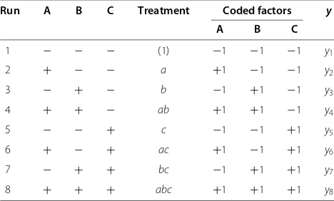
A 2kfactorial design involveskfactors, each at two levels. These levels can be quantitative or qualitative. The level of a quantitative factor can be associated with points on a numerical scale, as the size of population or the num-ber of islands. For qualitative factors, their levels cannot be arranged in order of magnitude, such as topologies, or strategies of selection. The two levels are referred as ‘low’ and ‘high’, and denoted by ‘−’ and ‘+’, respectively. It does not matter which of the factor values is associated with the ‘+’ and which with the ‘−’ sign, as long as the labeling is consistent.
At the beginning of a 2k factorial design, factors and levels are specified. When we combine them all, we get a design matrix. Table 1 shows the design matrix of the 23 factorial design.
For each combination of levels, also called treatment, the studied process is executed and the response variable yis collected.
After the data collection, the effects of factors can be calculated, and with appropriate statistical tests, we can determine whether the output depends in a significant way on the values of inputs. There are several excellent statistic software packages that are useful for setting up and analyzing 2kdesigns. In our experiments, we use the R [31] open source software environment for statistical computing and graphics.
Basically, the average effect of a factor is defined as the change in response produced by a change in the level of that factor averaged over the levels of the other factors. The two-way interactionABeffect is defined as the aver-age difference between the effect of factorAat the high level of factorBand the effect ofAat the low level ofB. The three-way interactionABCoccurs when there is any significant difference in two-way interaction plots corre-sponding to different levels of the third factor. For more details on this and other experimental designs, the reader is referred to [25,32].
Table 1 Notation of factors and level in a standard or Yates’ order for the 23factorial design
Run A B C Treatment Coded factors y
A B C
1 − − − (1) −1 −1 −1 y1
2 + − − a +1 −1 −1 y2
3 − + − b −1 +1 −1 y3
4 + + − ab +1 +1 −1 y4
5 − − + c −1 −1 +1 y5
6 + − + ac +1 −1 +1 y6
7 − + + bc −1 +1 +1 y7
Regression model of the 2kdesign
The results of the 2kfactorial design can be expressed in terms of a regression model. For the 22factorial design,
the effect full model is
y=β0+β1x1+β2x2+β12x1x2+ (9)
where y is the response, β are regression coefficients whose values are to be determined,xi are predictor vari-ables that represent coded factors levels:−1 and+1, and is the random error term. The method used to esti-mate the unknown coefficients β is the method of least squares [33].
Regression coefficients are related to effect estimates. The β0 coefficient is estimated by the average of all
responses. The estimates ofβ1 andβ2 are one half the
value of the corresponding main effect. In the same way, the interaction coefficients, asβ12, are one half the value of the corresponding interaction effect.
In regression, theR2 coefficient of determination is a statistical measure of how well the regression line approx-imates the real data points. AnR2of 1 indicates that the regression line perfectly fits the data. Theadjusted R2is almost the same asR2, but it penalizes the statistic as extra variables are included in the model.
Other measures have been developed to assess the model quality. The Akaike information criterion (AIC), the Chi-square test, the cross validation criterion, and others are methods used to compare models with different numbers of predictor variables [34]. These methods are useful in the model selection, one of the steps of the analy-sis of the 2kfactorial design (the ‘Analysis of the 2kdesign’ subsection) where it is verified whether all the poten-tial predictor variables are needed or a subset of them is adequate. The number of possible models grows with the number of predictors, which makes the selec-tion a difficult task. Presently, there are a variety of automatic computer search procedures to simplify this task [33].
This model requires some assumptions to be satisfied: the errors are normally and independently distributed withconstantvarianceσ2. Violations of the basic assump-tions and model adequacy can be easily investigated by the examination of residuals. Residuals are the differ-ence between observed values and estimated values. If the model is adequate, the residuals should be structureless. Any suggestion of a pattern may indicate other problems such as a model misspecification due to either nonlin-earity or the omission of important predictor variables, presence of outliers, and nonindependence of residuals.
The usual procedure for checking the normality assumption is to construct a normal probability plot of the residuals. If the underlying error distribution is nor-mal, this plot will resemble a straight line. The constant variance of error assumption is easily verified if we plot
the residuals versus the fitted values. This plot should not reveal any obvious pattern. To check for independence, in a plot of the residuals against time, if known, residuals should fluctuate in a more or less random pattern around the baseline zero.
Graphical analysis of residuals is inherently subjective, but frequently residual plots may reveal problems with the model more clearly than formal statistical tests. For-mal tests like the Durbin-Watson test (independence), Breusch-Pagan test (constant variance), and Shapiro-Wilk test (normality) can check the model assumptions [33]. More about formal tests in the ‘Implementation’ subsection.
If a violation of the model assumptions occurs, there are two basic alternatives: (1) abandon the linear regres-sion model and develop and use a more appropriate model, or (2) employ some transformation to the data. The first alternative may result in a more complex model than the second one. Sometimes, a nonlinear function can be expressed as a straight line using a suitable trans-formation. More on data transformation can be found in [25,33].
Analysis of variance
The analysis of variance (ANOVA) test is a statistical test which is used to compare means of two or more inde-pendent normal samples. It produces an F statistic that calculates the ratio of the variance among the means to the variance within the samples [33].
The ANOVA assumptions are the same as the regres-sion model assumptions described in the ‘Regresregres-sion model of the 2kdesign’ subsection. The ANOVA is robust to the normality assumption. If the assumption of homo-geneity of variances is violated, the ANOVA test is only slightly affected in the balanced (equal sample sizes in all treatments) fixed effect model. Lack of independence of error terms can have serious effects on the inferences in the analysis of variance [33].
Analysis of the 2kdesign
The statistical analysis of the 2k design follows the sequence of steps described:
1. Estimate factor effects. The factor effects are estimated, and their signs and dimensions are examined for a preliminary information regarding which factors and interactions may be important and in which directions these factors should be adjusted to improve the response.
2. Perform statistical testing. Many implementations of the2kfactorial design rely on replications where
each replicate represents a set of2kruns. When the
design is replicated, for a full model as in
There are other methods to determine which effects are nonzero. The standard error of the effects can be calculated, and then confidence intervals on the effects are established. Box et al. [32] state a rough rule: effects greater than two or three times their standard error are not easily explained by chance alone.
For an unreplicated design, there is a method due to Cuthbert Daniel [35], in which effects are plotted on a normal probability plot. The effects that are negligible are normally distributed with mean zero and varianceσ2and will tend to fall along a straight line on this plot. The significant effects will have nonzero means and will not lie along the straight line. An estimate of error can be obtained with the combined negligible effects. The formal tests of statistical significance are important to find out effects that are due to sampling error.
We should not confuse statistical significance with practical significance - whether an observed effect is large enough to matter. The statistical significance does not prove practical importance, but a practically significant effect should not be claimed unless it is statistically significant [14].
3. Refine the model. The model is adjusted as any nonsignificant factor can be removed from the model. 4. Check the model adequacy. The residual analysis is
performed to check for model adequacy and assumptions. If it is found that the model is inadequate or if assumptions are badly violated, it is necessary to refine the model (step 3).
5. Interpret results. When examining the magnitude and sign of the factor effects, we can determine which factors are likely to be important. The main effect of a factor should be individually interpreted only if there is no evidence that the factor interacts with other factors. If the interaction is present, the interacting factors must be considered jointly. The negative sign on an effect indicates that a change from low level− to high level+will reduce the response variable.
Results and discussion Implementation
The technical choices for the programming language and libraries are described in this section. Genetic algorithms (GA) are a widely used subfamily of EAs, which are stochastic search methods designed for exploring com-plex problem spaces in order to find optimal solutions using minimal information on the problem to guide the search.
We implemented a PGA with multiple populations following the island model (coarse-grained model). We named this implementation PGA-I. The population was divided into subpopulations, or islands, that evolve their
local population in parallel. One of them was called cen-tral process, and it controlled the synchronization of all other subpopulations.
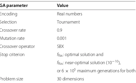
The parameters used in canonical GAs were kept fixed at the values shown in the Table 2 throughout the exper-imentation. The parameters related to the migration pro-cedure were varied. They are shown in Table 3.
The efficiency of C/C++compilers and the large num-ber of available libraries led us to choose C/C++ for coding. The known sensitiveness of GAs to the choice of the PRNG motivated the option to a high-quality PRNG [36]. We chose a combination of theSIMD-oriented Fast Mersenne Twister (SFMT) and the The Mother-of-All Random Generators (MoA) available in the A. Frog library [37].
For parallelization, we chose a Message Passing Inter-face (MPI) library called MPICH2 [38]. The MPICH2 is a message passing interface library with tested and proved scalability on multicores [39] and proved performance of message passing on shared memory [40].
The PGA-I was executed on a multicore Intel Xeon E5504, with two CPUs, four cores each at 2 GHz, 256-KB cache L2, 4-MB cache L3, FSB at 1,333 MHz, 4 GB, Ubuntu 10.04 LTS (kernel 2.6.32).
The data analysis was performed using R, the free soft-ware environment for statistical computing and visualiza-tion [31]. The following formal statistical tests available in R were employed: the Shapiro-Wilk test of normal-ity, shapiro.test from thestatspackage [31]; the Breusch-Pagan test of constant variance,ncvTestfrom the car package [41]; and the Durbin-Watson test of independence,dwtestfrom thelmtestpackage [42].
Case studies
The goal of our experimentation was to find out which of the factors that affects the speedup of the PGA-I the most when solving the selected test functions (see the ‘Test functions’ subsection). We selected seven factors
Table 2 Fixed canonical parameter settings
GA parameter Value
Encoding Real numbers
Selection Tournament
Crossover rate 0.9
Mutation rate 0.001
Crossover operator SBX
Stop criterion fRas: optimal solution and
fRos: near-optimal solution (10−10),
or 6×10⁵maximum generations for both
Problem size 30 dimensions
Table 3 Factors and levels
Id Factors Coded levels
High level (+) Low level (−)
Proc Number of islands 4 16
Top Topology Single ring All-to-all
Rate Migration frequency 10 100
Pop Population size 1,600 3,200
Nindv Amount of migrants 1 5
Sel Selection strategy Random Best fitted
Rep Replacement strategy Random Worst fitted
related to the migration parameters to investigate, as described in Table 3.
The 27factorial design matrix was built as described in
the ‘2k Factorial design’ subsection, with two additional lines related to sequential execution times, each with the population size of 1,600 and 3,200 individualsa. It adds up to 130 different configurations to be tested. A PRNG was used to determine the execution order and, for each treat-ment, the wall clock execution time was captured. As the speedup requires an estimate of sequential and parallel times, we replicated the experimentntimes. We started withn=40, and it was increased when necessary.
The conditions of the speedup ratio distribution to approximate to a normal distribution, as established in the ‘Ratio of two independent normal random variables’ sub-section, were checked. If the conditions were not satisfied, the number of replications was increased and the condi-tions were verified again. Then, the analysis of the 27
fac-torial design, as described in the ‘Analysis of the 2kdesign’ subsection, was performed. The statistical significance level of 0.05 and the practical significance of effects larger than 10% of the average speedup were considered in our analysis.
The following notation is used in this work: we denoted the two sets of sequential execution times byXpj, wherep is the population size andjis the replicate, and denoted the 128 sets of parallel execution times by Yij, wherei is the treatment number and j identifies the replicate. Sample means and sample standard deviations were used on estimated coefficients of variationδˆ.
This procedure was performed for each test function, as described in the ‘Rosenbrock function - 27 factorial
design’ and ‘Rastrigin function - 27 factorial design’
subsections.
Test functions
The selected test functions are well known and have been used in benchmarks, such as the CEC 2010 [43]. They are the Rastrigin function (fRas) and the Rosenbrock function
(fRos). The former is one of the De Jong test functions and
Table 4 Sequential execution times summary - Rosenbrock function
Pop Minimum First Median Mean Third Maximum
quartile quartile
1,600 216,867 218,285 219,202 219,153 219,752 223,377
3,200 426,218 430,814 431,824 431,861 433,025 435,554
is relatively easy for GAs to solve. It is a nonlinear mul-timodal and separable function with a large number of local minima. The latter is a nonseparable function, and its global minimum is inside a long, narrow, parabolic-shaped flat valley. Even though it is trivial to find the valley, to converge to the global minimum is difficult.These func-tions were chosen by their different characteristics, and the experiments yielded different results for both.
The test function formulas are given:
fRas(X)=10q+ q
i=1
(x2i −10 cos(2πxi)), (10)
where q is the dimension, −5.12 ≤ xi ≤ 5.12, and its global minimum isfRas(X∗) = 0, andX∗ =[ 0, 0,. . ., 0].
We tested it with 30 dimensions (q=30).
fRos(x)= q−1
i=1
(1−xi)2+100(xi+1−x2i)2
, (11)
whereqis the dimension,−2.0≤xi≤2.0, and its global minimum isfRos(X∗) = 0, and X∗ = [ 1, 1,. . ., 1]. We
tested it with 30 dimensions (q = 30) and searched for a near-optimal solution equal or less than 10−10.
Rosenbrock function - 27factorial design
The 27 factorial design plus two treatments for the sequential executions were replicated 40 times. It con-stituted a matrix with 40 columns and 130 lines filled with execution times. The execution times added up to approximately 120.4 h.
Table 4 presents statistics of the sequential execution times for each population sizes. Both estimated coeffi-cients of variationδˆX1600andδˆX3200were lower than 0.2.
For theYijparallel execution times, the maximum val-ues of δˆYi was 0.297, and the maximum value of δˆY
i
was 0.047. All δˆY
i were under 0.2, as recommended in
the ‘Ratio of two independent normal random variables’
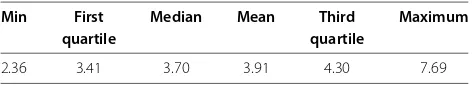
Table 5 Speedup summary - Rosenbrock function
Min First Median Mean Third Maximum
quartile quartile
Table 6 Factor levels for the lowest and highest observed speedup - Rosenbrock function
Id Factors Lowest speedup Highest speedup
Proc Number of islands 16 16
Top Topology Single ring All-to-all
Rate Migration frequency 100 10
Pop Population size 1,600 3,200
Nindv Amount of migrants 1 1
Sel Selection strategy Best fitted Best fitted
Rep Replacement strategy Worst fitted Worst fitted
subsection. The conditions established by Theorem 1 were satisfied. Thus, the distribution of the speedups, calculated by the weighted ratio formula (4), had an approximation to a normal distribution.
The summary shown in Table 5 gives a mean speedup of 3.91. There were 14 superlinear speedups observed for the PGA-I running on four islands.
The lowest and the highest speedups were observed when factors Proc, Top, Rate, Pop, Nindv, Sel, and Rep were set at+ − + − − + +and+ + − + − + +levels, respectively, as shown in Table 6.
At first, there was one speedup estimate for each treat-ment, and we had an unreplicated factorial. We started by assuming that all four-factor and higher interaction terms are unimportantb. The estimated effects of the
third-order model of the 27unreplicated factorial design were
–
–
– –
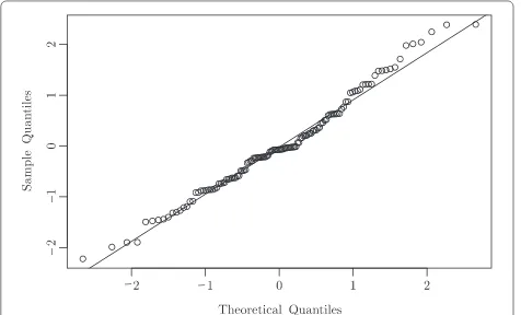
Figure 1Normal probability plot of the estimated effects of the 27factorial design - Rosenbrock function.
displayed in a normal probability plot. The significant effects are identified in Figure 1.
The factor Rep and all interaction involving Rep were negligible. We dropped the factor Rep from the experi-ment. The design became a 26factorial with two
repli-cations. The projection of an unreplicated factorial into a replicated factorial in fewer factors is called design projection [25].
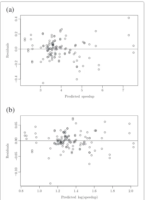
The analysis of the residuals of the third-order linear model for the 26factorial design revealed that the spread of the residuals was increasing as the predicted speedup values get larger, an indication of nonhomogeneity vari-ance, shown in Figure 2a. The Breusch-Pagan test [44] confirmed that the error variance changes with the level of the predicted speedup.
A log transformation of the speedup was performed, where y∗=log(y). For the log-transformed speedup model, the residual versus predicted value plot is shown in Figure 2b.
Following the log data transformation, an automatic search procedure for model selection based on the AIC criterion was performed. Table 7 presents the adjusted
(a)
(b)
–
–
–
–
Figure 2Residual versus predicted value plot for third-order model for the 26factorial design - Rosenbrock function.
Table 7 Adjusted linear regression model for the 26
factorial design following log data transformation -Rosenbrock function
Estimate Standard error tvalue Pr(>|t|)
(Intercept) 1.338 0.0035 385.842 <2e−16
Top 0.098 0.0035 28.141 <2e−16
Pop 0.096 0.0035 27.677 <2e−16
Rate −0.095 0.0035 −27.481 <2e−16
Sel 0.075 0.0035 21.558 <2e−16
Nindv 0.029 0.0035 8.223 5.98e−13
Proc 0.018 0.0035 5.114 1.45e−06
Rate:Sel −0.054 0.0035 −15.616 <2e−16
Top:Sel 0.021 0.0035 5.998 2.93e−08
Top:Proc 0.066 0.0035 19.125 <2e−16
Pop:Proc 0.055 0.0035 15.785 <2e−16
Rate:Proc −0.041 0.0035 −11.726 <2e−16
Top:Rate −0.017 0.0035 −5.039 1.98e−06
Top:Pop −0.014 0.0035 −4.045 0.0001
Sel:Proc 0.014 0.0035 3.940 0.0001
Top:Nindv −0.013 0.0035 −3.662 0.0004
Rate:Nindv −0.012 0.0035 −3.511 0.0007
Sel:Nindv 0.010 0.0035 2.740 0.0072
Pop:Rate 0.008 0.0035 2.308 0.0230
Top:Rate:Sel −0.015 0.0035 −4.305 3.80e−05
Rate:Sel:Proc −0.012 0.0035 −3.522 0.0006
Top:Pop:Proc −0.011 0.0035 −3.075 0.0027
Top:Sel:Nindv −0.010 0.0035 −2.934 0.0041
Top:Rate:Proc −0.008 0.0035 −2.183 0.0313
regression model for the 26 factorial design following the log data transformation. The adjusted model with all significant terms is given by
y∗=1.338+0.018x1+0.098x2−0.095x3+0.096x4
+0.029x5+0.075x6−0.054x3x6+0.021x2x6 +0.066x2x1+0.055x4x1−0.041x3x1 −0.017x2x3−0.014x2x4+0.014x6x1 −0.013x2x5−0.012x3x5+0.010x6x5 +0.008x4x3−0.015x2x3x6
−0.012x3x6x1−0.011x2x4x1 −0.010x2x6x5−0.008x2x3x1,
(12)
where the coded variables x1, x2, x3, x4, x5, and x6
represent factors Proc, Top, Rate, Pop, Nindv, and Sel,
(a)
(b)
–
–
–
–
– –
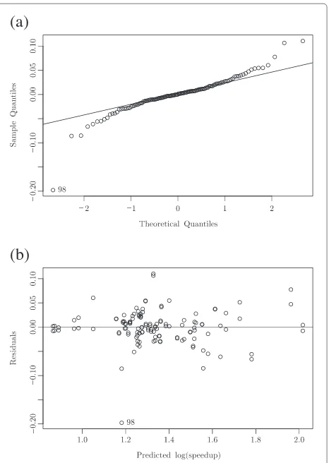
Figure 3Residual analysis for the adjusted model
(12) - Rosenbrock function.(a)Normal probability plot of residuals. (b)Plot of residuals versus predicted log (speedup).
respectively. This model presented a residual standard error equal to 0.0392 on 104 degrees of freedom, the coef-ficient standard error was 0.00347, and theR2was 0.975, which means the factors and interactions in the model explained approximately 98% of the variation iny∗. The adjustedR2was 0.969.
’
’
Figure 5Bar plot of the back-transformed estimated effects for the adjusted model (12) - Rosenbrock function.
Figure 3 presents the normal probability plot of resid-uals and the plot of residresid-uals versus predicted values. No unusual structure was apparent, and most of the residuals in the normal probability plot resembled a straight line, apart from residual 98.
Formal tests of equality of variances and normality and independence for the reduced model were executed. At a significance level of 0.05, the Breusch-Pagan test (pvalue = 0.24) could not reject the hypothesis that the residuals have a homogeneous variance, and the Durbin-Watson test (p value = 0.26) also could not reject the hypothesis that the residuals are independent. However, the Shapiro-Wilk test (pvalue=6.851e−08) rejected the hypothesis that the errors are normally distributed.
Moderate departures from normality are of little con-cern in the fixed effect analysis of variance, though outlying values need to be investigated [25]. Formal tests to aid in evaluation of outlying cases have been developed, such as the Cook’s distance, the studentized residuals and the Bonferroni test [33]. We run the R
functionoutlierTestfrom thecarpackage [41], and residual 98 had the Bonferroni adjusted pvalue<0.05. Figure 4 shows the that residual 98 had the largest Cook’s distance.
The adjusted model made without observation 98 showed that the inferences were not essentially changed. Observation 98 did not exercise undue influence so that no remedial measure was performed. We concluded that the model fory∗given by Equation (12) was satisfactory, and we could estimate the speedup using back transfor-mation given byy=ey∗.
The log transformation has a multiplicative interpreta-tion, e.g., adding 1 to log(y)multipliesybye, whereeis approximately 2.72. The bar plot of the statistically and practically significant back-transformed estimated effects for the adjusted model is displayed in Figure 5.
Discussion The effect of Nindv and its interactions were smaller than 10%, which is statistically but not practi-cally significant. This could be due to the small difference between the high and low levels of Nindv. The high level was defined as five individuals based on the high level of number of islands, population size, and migration topol-ogy. When there were 16 islands and 1,600 total popula-tion size, each island had 100 individuals. If the topology was the all-to-all type, each island would receive a num-ber of migrants equal to the numnum-ber of islands versus the number of migrants. This calculation should be less than the island population.
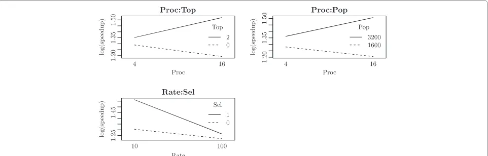
The two-factor interactions, namely Proc:Top, Proc: Pop, and Rate:Sel, were statistically and practically signifi-cant. They are shown in Figure 6.
The effect of the Proc:Top interaction was 0.133 on log(speedup), i.e., 14.2% speedup increase. With Proc set at the low level with four islands, the speedup was increased by 6.5% when Top changed from the ring to all-to-all topology. With Proc set at the high level with 16
Table 8 Summary of sequential execution times for 1,000 replicates - Rastrigin function
Pop Minimum First Median Mean Third Maximum
quartile quartile
1,600 2,544 2,672 2,699 6,770 2,729 551,307
3,200 5,112 5,309 5,351 5,358 5,397 6,516
islands, the change from ring to all-to-all topology had the effect of 38.8% increase on the speedup.
The factors Proc and Pop interacted with effect size of 11.6% speedup raise. With Proc set to four islands, speedup increased by 8.6% as Pop modified from 1,600 to 3,200 individuals. When Proc was 16 islands, speedup increased by 35.2% as Pop changed from 1,600 to 3,200 individuals.
The effect of Rate:Sel interaction was a 10.3% speedup decrease. At the low level of Rate, migration at every 10 generations, the speedup increased by 29.4% when Sel changed from random to best-fitted selection strategy. With Rate set to 100 generations, the speedup increased by 4.2% when factor Sel changed from low to high level.
Some of the three factor interactions were statistically significant, but their effects had a small influence on the speedup, which was less than 10%.
Rastrigin function - 27factorial design
The 27 factorial design plus two treatments for the sequential executions were replicated 40 times. It consti-tuted a matrix with 40 columns and 130 lines filled with execution times. The execution times added up to approx-imately 21.3 h. The conditions to the ratio distribution to approximate to a normal distribution were checked.
The estimated δˆX1600 was >1. Thus, it did not satisfy
Theorem 1. For the parallel execution times, the esti-matedδˆYi ranged from 0.014 to 4.998 and the estimated
ˆ δY
iranged from 0.020 to 0.790. SomeδˆYiwere higher than
the recommended limit of 0.2 (see the ‘Ratio of two inde-pendent normal random variables’ subsection). There was no guarantee of the existence of a normal approximation to the distribution of the speedup.
A sample of a sufficiently large size reduces δY
n. The
estimator of the sample size is given by Equation (5). We applied this to the Yij sample and found ns>624. Although some of theYi have a small coefficient of vari-ation, the full factorial was replicated 1,000 times and the
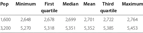
Table 9 Summary of sequential execution times after the removal of extreme values - Rastrigin function
Pop Minimum First Median Mean Third Maximum
quartile quartile
1,600 2,648 2,678 2,699 2,701 2,722 2,764
3,200 5,270 5,318 5,351 5,352 5,385 5,453
Table 10 Speedups summary - Rastrigin function
Minimum First quartile Median Mean Third quartile Maximum
0.01 0.65 3.04 2.32 3.65 4.85
data were kept balanced. The execution times added up to approximately 438 h.
The analysis of the 1,000 replicates of the 27 factorial design produced theXpsummary statistics presented in Table 8. X1600 showed extremely high values that were
unusually far from other observations. Extreme values could also be seen among Yi. The mean is not robust to extreme values. It is affected more by outliers than the median. According to [45], the mean exploits the sample because it gives equal weight to each observa-tion. Contrarily, the median is resistant to several outlying observations since it ignores a lot of information.
The trimmed mean is a robust estimator of central ten-dency. To find a trimmed mean, thex% largest and small-est observations are deleted, and the mean is computed using the remaining observations. In fact, the median is just a trimmed mean with the percentage of trim equal to 50% [46].
We applied the trimmed mean with the percentage of trim equal to 10% to estimateXp andYiin the speedup estimation. This procedure was equivalent to sortXpand Yiobservations and discarded 10% of the smallest and 10% of the largest values from each one.
Table 9 presents the summary statistics for Xp after the trimming procedure. The estimated coefficients of variation δˆXp and δˆXp were under 0.0107 and 0.0004,
receptively. The estimated coefficients of variationδˆYiand ˆ
δY
i were under 1.529 and 0.0541, respectively. These
val-ues did not satisfy the conditions stated in Theorem 1, but they satisfied the condition of δˆY
i being under 0.2,
described in the ‘Ratio of two indepen- dent normal ran-dom variables’ subsection. The weighted ratio given by Equation (4) was preferable to estimate the speedup. The mean speedup of all 128 observations was 2.32, as shown in Table 10.
Table 11 Factor levels for the lowest and the highest observed speedup - Rastrigin function
Id Factors Lowest speedup Highest speedup
Proc Number of islands 16 16
Top Topology Single ring All-to-all
Rate Migration frequency 100 10
Pop Population size 1,600 3,200
Nindv Amount of migrants 1 5
Sel Selection strategy Random Random
–
–
– –
Figure 7Normal probability plot of the estimated effects of the 27factorial design - Rastrigin function.
There were 38 sublinear speedups, all of them occurred when running on 16 islands, and two superlinear speedups when running on four islands. The lowest and the highest speedups were observed when factors Proc, Top, Rate, Pop, Nindv, Sel, and Rep were set at+ − + − − − −and+ + − + + − +levels, respectively, as shown in Table 11.
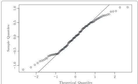
Then, we proceeded to the analysis of the unreplicated 27factorial design. Figure 7 presents the normal
probabil-ity plot of the estimated effects.
The factor Rep and all interactions involving Rep were negligible. We dropped the factor Rep from the experiment. The design became a 26 factorial with two replicates.
–
–
Figure 8Plot of residuals versus predicted speedups for the third-order model for 27factorial design - Rastrigin function.
–
–
– –
Figure 9Normal probability plot of residuals for the 26factorial design - Rastrigin function.
Figure 8 shows the plot of residuals of the third-order model 26 factorial design against the predicted values. The residuals looked structureless. The normal probabil-ity plot of the residuals resembled a straight line, as shown in Figure 9.
From the third-order linear regression model for the 26
factorial design, an automatic search procedure for model selection based on the AIC criterion resulted in the model described in Table 12. The adjusted model was built as follows:
y=2.318−0.816x1+0.327x2−0.269x3+0.529x4 +0.296x5+0.320x2x3,
(13)
where the coded variables x1, x2, x3, x4, and x5
repre-sent factors Proc, Top, Rate, Pop, and Nindv, respectively. This model presented a residual standard error of 0.978 on 121 degrees of freedom, andR2was 0.593, which means that the model explained 59% of the variation ofy. The adjustedR2was 0.573.
Formal tests of equality of variances, normality, and independence on the reduced model were executed. The Shapiro-Wilk test (pvalue=0.13), the Breusch-Pagan test (pvalue=0.06), and the Durbin-Watson test
Table 12 Third-order linear regression model for the 26 factorial design - Rastrigin function
Estimate Standard error tvalue Pr(>|t|)
(Intercept) 2.318 0.0864 26.821 < 2e−16
Proc −0.816 0.0864 −9.445 3.38e−16
Pop 0.529 0.0864 6.121 1.19e−08
Top 0.327 0.0864 3.789 0.0002
Nindv 0.296 0.0864 3.423 0.0008
Rate −0.269 0.0864 −3.110 0.0023
–
–
Figure 10Plot of residuals versus predicted speedups for the adjusted model (13) - Rastrigin function.
(pvalue=0.20) did not reject the null hypotheses of nonnormality, nonhomogeneity and nonindependence of residuals, respectively.
Figure 10 presents a plot of the residuals versus pre-dicted speedup, and Figure 11 presents the normal proba-bility plot of the residuals for this adjusted model. Though the formal tests did not indicate any problem, Figure 10 shows some nonlinear pattern. The small coefficient of determinationR2also corroborated that the model might be improved if higher order terms were added to the model or other predictor variables were considered. The bar plot of the absolute value of the estimated effects is presented in Figure 12. All effects were practically signif-icant because they were higher than 0.23, i.e., 10% of the mean speedup.
Discussion The factor Proc had the largest main effect of −1.63. Changing Proc from 4 to 16 islands dropped the mean speedup by 1.63. Factor Pop had the second largest main effect of 1.06. If the population size increased from 1,600 to 3,200, the speedup increased by 1.06. The
–
–
– –
Figure 11Normal probability plot of residuals for the adjusted model (13) - Rastrigin function.
Figure 12Bar plot of the absolute estimated effects for the adjusted model (13) - Rastrigin function.
main effect of Nindv was 0.6. The speedup increased when the number of migrants changed from one to five.
The effect of interaction Top:Rate was 0.64, and it is shown in Figure 13. With factor Top set to ring topology, when Rate changed from 10 to 100 generations, the mean speedup dropped by 1.18. With factor Top set to all-to-all topology, the mean speedup increased by 0.10 as the Rate changed from 10 to 100 generations.
Rastrigin is a multimodal function, and it presented exe-cution times with higher coefficient of variation when compared to the Rosenbrock function. This variability affects the sharpness of the statistics, and a larger number of replicates was necessary. This was also reflected on the higher error estimates.
The execution times of PGA-I on solving the Rastri-gin function presented some extreme execution times. We investigated these outlying values, and we could repro-duce them using the same PRNG seed. They were not
due to erroneous measures, failures of registry, or exter-nal perturbations. By trimming them, we were effectively discarding information about the best and worst perfor-mances of the algorithm. The distribution of the execu-tion times were also changed. This is a limitaexecu-tion of our method.
Conclusions
This paper introduced a method to guarantee the correct estimation of speedups and the application of a factorial design on the analysis of PEA performance. As a case study, we evaluated the influence of migration related to parameters on the performance of a parallel evolutionary algorithm solving two benchmark problems executed on a multicore processor. We made a particular effort in care-fully applying the statistical concepts in the development of our analysis.
The performance and the factor effects were not the same for the two benchmark functions studied in this work. The Rastrigin function presented higher coefficient of variation than the Rosenbrock function, and the factor and interaction effects on the speedup of the PGA-I were different in both.
Further work will be done on the high variability of the results yielded by the algorithms tested. We observed extreme values in the execution times of PGA-I when solving the Rastrigin function, in the ‘Rastrigin function - 27factorial design’ subsection. These extreme measures were investigated, and they could be reproduced by applying the same seed.
We intend to study alternative approaches to deal with extreme values. One approach is to perform a rank trans-formation [47]. Another option is to block the PRNG seed to isolate its influence on the variability of execution times. Blocking the seed is a controversial subject: it is a statistically sound approach, but it is not a common prac-tice to specify the seed that is used in the execution of EAs. EAs are usually executed several times with different seeds to get a sense of the robustness of the procedure. The seed effects may be of little relevance to the EA community. Future works demand a proper investigation of this issue.
Endnotes
aThe population size is one of the investigated factors
with two levels: 1,600 and 3,200 individuals. It is important to ensure the same workload conditions for both sequential and parallel times. Thus, it is necessary to capture the sequential times for these two population sizes and to have the same population size for the sequential and the parallel times in the speedup ratio.
bThe sparsity of the effect principle states that a system
is usually dominated by main effects and low-order interactions, and most high-order interactions are negligible [25].
Competing interests
The authors declare that they have no competing interests.
Authors’ contributions
MSP carried out the background and literature review, implemented the parallel genetic algorithm, conceived the design of experiments, performed the statistical analyses and drafted the manuscript. ISP participated in the implementation of the parallel genetic algorithms and in the design of experiments, and helped to draft the manuscript. KY was involved in conceiving of the study and participated in its design. ERP participated in the design of the experiments and the statistical analyses, and helped to draft the manuscript. All authors read and approved the final manuscript.
Acknowledgements
We would like to thank the anonymous referees whose really careful reading, useful comments, and corrections have led to significant improvement of our work. Mônica S Pais and Igor S Peretta were partially supported by
IFGoiano/FAPEG/CAPES and CNPq, respectively.
Author details
1Department of Informatics, Goiano Federal Institute of Education, Science and Technology (IFGoiano), Campus Urutaí, Rodv. Geraldo Silva km 2,5, Urutaí, Goiás 75790-000, Brazil.2Faculty of Electrical Engineering, FEELT, Federal University of Uberlândia (UFU), Uberlândia, Minas Gerais 38400-902, Brazil. 3Faculty of Mathematics, FAMAT, Federal University of Uberlândia (UFU), Uberlândia, Minas Gerais 38408-100, Brazil.
Received: 29 November 2013 Accepted: 2 December 2013 Published: 3 February 2014
References
1. Chiarandini M, Paquete L, Preuss M, Ridge E (2007) Experiments on metaheuristics: methodological overview and open issues. Technical report DMF-2007-03-003 The Danish Mathematical Society 2. Cantú-Paz E (2000) Efficient and accurate parallel genetic algorithms.
Kluwer Academic Publishers, Norwell
3. Tomassini M (2005) Spatially structured evolutionary algorithms: artificial evolution in space and time (natural computing series). 1st edn. Springer, Secaucus
4. Alba E (2002) Parallel evolutionary algorithms can achieve super-linear performance. Inf Process Lett 82(1): 7–13
5. Kim H, Bond R (2009) Multicore software technologies. IEEE Signal Process Mag 26(6): 80–89
6. Diaz-Frances E, Rubio F (2013) On the existence of a normal
approximation to the distribution of the ratio of two independent normal random variables. Stat Pap 54(2): 309–323
7. Qiao CG, Wood GR, Lai CD, Luo DW (2006) Comparison of two common estimators of the ratio of the means of independent normal variables in agricultural research. J Appl Math Decis Sci 2006.
doi:10.1155/JAMDS/2006/78375
8. Eiben AE, Smith SK (2011) Parameter tuning for configuring and analyzing evolutionary algorithms. Swarm and Evol Comput 1: 19–31
9. Touati S, Worms J, Briais S (2012) The speedup-test: a statistical methodology for programme speedup analysis and computation. Concurrency and Comput: Practice and Experience 25(10): 1410–1426 10. Alba E, Luque G, Nesmachnow S (2013) Parallel metaheuristics: recent
advances and new trends. Int Trans Oper Res 20(1): 1–48. doi:10.1111/j.1475-3995.2012.00862.x.
11. Coy SP, Golden BL, Runger GC, Wasil EA (2001) Using experimental design to find effective parameter settings for heuristics. J Heuristics 7: 77–97. 10.1023/A:1026569813391
12. Czarn A, MacNish C, Vijayan K, Turlach BA, Gupta R (2004) Statistical exploratory analysis of genetic algorithms. Evol Comput, IEEE Trans 8(4): 405–421. doi:10.1109/TEVC.2004.831262
13. Bartz-Beielstein T (2006) Experimental research in evolutionary computation: the new experimentalism (natural computing series). 1st edn. Springer, Secaucus