19 3, XX, 2017
DOI: 10.15240/tul/001/2017-3-002
Introduction
In the economic, econometric and demographic literature, there coexist a few concepts, seemingly similar but signifi cantly different, whose purposes are predictive, intended to restructure and optimize, but also from a natural scientifi c need to know, understand, predict or prevent processes and systems; such concepts as forecasting, estimation, designing, assessing, planning, prediction and prospecting (Săvoiu, 2007, p. 351) and, last but not least, the simulation.
Prognosis and prediction arose from the need to anticipate the trends of evolution of the terms of a chronological series of data, and are refl ected in the examination of the trend, the periodic oscillations and the purely random component, following the contour of the cycle of the primary phenomenon of the past period, and also in identifying the factors of signifi cant action in the future. The fi rst concept, prognosis, originally defi ned a form of pre-knowledge or anticipation of the evolution in time of a number of processes and systems, further characterized by more objectivity and scientifi c integrity, with practically reproducible valences, and generated an integrated set of methods and specifi c techniques. A recognized aspect, which was frequently proved by the accuracy of prognoses or forecasts, is that the accuracy of its results depends on the quality of data analysis and subsequent errors, as well as the quality of the hypotheses. Prediction is a term taken over from French statistics and demography, and had a more subjective and intuitive conceptual outline, also having even accents of non-reproducibility when defining the likelihood or the subsequent emergence or evolution of processes and systems (demographic, economic, social, etc.) in the analysis of certain information owned at a certain time (Kucharavy & De Guio, 2005; 2012).
Even if one very carefully chooses the terms forecast, prediction, or projection, there immediately arise other necessary options, as the concept will be accompanied by a new defi ning characteristic: exploratory, tendential, oscillatory, normative, global, analytical, fundamental, sequential etc. Planning, projection and estimation lend various nuances to the analysis of the process and system, drawing on hypotheses that are structural or mostly internal to the system, and prediction, which „presupposes reaching a temporal target, towards which an economic phenomenon converges“ (Săvoiu, 2016), is focused on the outcome of the extended process or system, involving the action of their external factors as well. If the prospect or perspective admits to hold perhaps the vaguest contour of the future, encompassing the real to a signifi cant extent, no less than the potential (which sometimes becomes even fi ctional), prospection or prospectology complements the sense of prediction or forecast in the spirit of quantifi cation and the action undertaken in order to achieve it (with rigorous evaluations of the prospecting errors).
Defi ned as „scientifi c method, research or teaching technique that reproduces actual events and processes under test conditions; developing a simulation is often a highly complex mathematical process. Initially a set of rules, relationships, and operating procedures are specifi ed, along with other variables“ in Encyclopaedia Britannica (2012), simulation was preferred by the authors, starting from its ability to provide a complex macro-fi nancial forecast of probable future funds (revenues), but also the benefi ts provided by any software developed with the purpose of simulation, which is focused on modelling real processes, from mathematical transposition, and fi nalized by testing statistical hypotheses and validations/
A MONTE CARLO METHOD SIMULATION
OF THE EUROPEAN FUNDS THAT CAN BE
ACCESSED BY ROMANIA IN 2014-2020
Gheorghe S
ă
voiu, Emil Burtescu, Vasile Dinu, Ligian Tudoroiu
EM_3_2017.indd 19
20 2017, XX, 3
invalidations of models of certain usefulness and effective optimization valences, and clear utility in establishing major fi nancial programs or plans, as well as the budgets related tot hem (Maverick, 2016). The essential steps of the simulation, which were pursued in this article, were connected with: a) problem defi nition, conceptual selection and design of the study/research; b) defi nition and development of the probabilistic model of the economic process; c) the choice of the method, formulation of hypotheses, the defi nition of variables and effecting the economic simulation process; d) the initial calibration of the simulation of the economic process; e) the statistical analysis of the simulation (including predictability, sensitivity and accuracy, or error level); f) the implementation of the results of the simulation, identifying the limits of the process, also when modifying the procedural reality, the specifi cation of the need to regularly re-develop the model, etc.
The reminder of the paper is classical and quite succinct, as a brief conceptual introduction is followed by a section devoted to the funds accessed by Romania from the European Union (EU), as a modelled process, then there is the description of the method of simulation used (i.e. Monte Carlo), and also the formulation of hypotheses, scenarios and variables. The simulation results are presented and discussed separately in the article, and a set of conclusions, limitations and perspectives conclude the articulated approach of the research.
1. Value and Absorption Rate of the
European Funds Accessed by
Romania in the First Budget
Period (2007-2013), and the First
Two Years of the Second One
One of the major problems of the Romanian economy is closely linked, among other things, to its tendency to absorb European funds (Săvoiu et al., 2006). In the fi rst fi nancial or budget period of the European funds for Romania, between 2007 and 2013, according to latest available data, the national economy recorded, in all the three indicators or all the specifi c absorption rates, values placed well below the EU average – by around 10% on average (with an effective rate of 79.23%, a current absorption rate of 82.93%, and an overall absorption rate of 90.44%, which also includes the amounts received from the EU in advance, as of 31st January 2017). At the end of 2015, the gap was more than 20% (69.9%, compared to the European average of 89.9%), and the sustained efforts in 2016 have halved that gap. The effective absorption of the fi rst EU budget period, detailed by operational programs, is placed within a range of values going from 73.37% to 86% (Tab. 1). The same structure for the period 2014-2020 is marked by changes centred on the regional expansion and human capital development, while there is a contraction of the funds allocated to competitiveness:2014-2020 2007-2013
Operational programs mil. euro Operational programs mil. euro
Effective absorption
rate % Regional development 6,600.00 Regional development 3,966.02 85.04 Large infrastructure
9,418.52
Environment 4,412.47 78.48
Transportation 4,288.13 74.63
Competitiveness 1,329.79 Competitiveness 2,536.64 85.94
Human capital 4,326.84 Human resources 3,476.14 73.37
Development of administrative
capacity 553.19
Development of administrative
capacity 208.00 82.00
Technical assistance 212.77 Technical assistance 170.23 86.00 Helping disadvantaged people 441.00
Total 22,882.11 Total 19,057.65 79.23
Source: own based on Annual Fiscal Report, 2015 (http://www.consiliulfi scal.ro/RaportanualCF2015.pdf)
Tab. 1: European funds allocated to Romania in 2014-2020 and 2007-2013
EM_3_2017.indd 20
21 3, XX, 2017
Comparing the overall absorption to the current rate, the latter has more polarized structural values, namely from a minimum of 73.37% to 113.42%, outlining possible hypotheses and scenarios for boosting the funds that can be accessed from the EU by Romania’s economy, in the period 2014-2020 (Tab. 2).
Useful information for the simulation or annual forecast of the funds that can be accessed by Romania in the future occur in the absorption rate confronted with the EU average for the last period 2007-2013 (Fig. 1).
The EU’s new budget period, as far as the accessing of European funds is concerned, is placed within trends similar to the one above,
Operational programs CAR EAR GAR (in advance)
Regional development – POR 85.04 85.04 93.50
Environment – POS 78.55 78.49 90.29
Transportation – POS 77.31 74.63 86.88
Competitiveness – CCE POS 105.47 85.94 95.00
Human resources – POS DRU 73.37 73.37 87.49
Developing administrative capacity – PODCA 98.66 82.00 95.00
Technical assistance – POAT 113.42 86.00 95.00
Total 82.93 79.23 90.44
Sources: own based on http://www.fonduri-ue.ro/21-transparenta/stadiul-absorbtiei/26-stadiul-absorbtiei and http://www.consiliulfi scal.ro/RaportanualCF2015.pdf
Tab. 2: Current Absorption Rate – CAR, Effective Absorption Rate – EAR and General Absorption Rate – GAR (2007-2013) in Romania (%)
Fig. 1: The Romanian national rate of absorption compared with the European annual average in the period 2007-2013 (including reports from 2014 to 2016)
Source: oown based on http://www.consiliulfi scal.ro/RaportanualCF2015.pdf Note: Software used EViews
EM_3_2017.indd 21
22 2017, XX, 3
only it has a much lower initial level in the fi rst three years, both in Romania and in the EU (Fig. 2).
Some statistical aspects characteristic of the fi rst EU fi nancial period, in which Romania is also participating as a member state, compared to the specifi cs of the EU average, describe an annual evolutionary heterogeneity, according to a coeffi cient of uniformity of the
annual absorption rate of 72.8%, a tendency to asymmetry and a modal placement completely opposite to the average absorption trend of the European funds (Fig. 3), in parallel with signifi cant gaps, completely opposite during the initial and fi nal absorption (the right-hand graph identifi es a transformation of the gap into an advance, since 2013, in favour of Romania). Fig. 2: The Romanian annual absorption rate compared with the European annual average in 2014-2016
Source: own based on http://www.fonduri-ue.ro/21-transparenta/stadiul-absorbtiei/26-stadiul-absorbtie
RO EU
Mean 9.259000 9.300000
Median 7.350000 10.525000
Maximum 18.690000 16.100000
Minimum 2.200000 1.980000
Std. Dev. 6.741375 4.776861
Skewness 0.309213 -0.318353
Kurtosis 1.421116 1.796645
Jarque-Bera 1.198051 0.772274 Probability 0.549347 0.679677
Sum 92.590000 93.000000
Sum Sq. Dev. 409.015300 205.365600 Observations 10.000000 10.000000
Source: Source: The annual data for the effective rate of absorption of EU and RO were processed by the authors with the software package EViews
Fig. 3: Descriptive statistics of the data series of annual absorption rate in the period 2007-2016, and recuperative dynamics of gaps (RO–EU)
EM_3_2017.indd 22
23 3, XX, 2017
Unfortunately, the effort of making up for the absorption lags between RO and EU outlines not only two normal distributions that are completely opposite, as a dominant of small and large ratios, Skewness, Kurtosis and impact of the modal area (Fig. 4), but also a weak link, in keeping with the value of the specifi c ratio R in the correlation matrix, with predictive valences, between the dynamics of the absorption rate in the EU and in RO (Tab. 3).
Although invalidated by testing (F-statistic = 1.654, compared with F-theoretical = 4.96 for α = 0.05), due to the small number of years in the fi rst budget cycle (10 terms), the relationship between the two variables remains of the type “bidirectional and iterative, given by the simultaneity of interaction and adaptation of specifi c factors” (Krivokapić & Jaško, 2015),
and can delineate, in future, a correlation able to generate, by using the software package EViews, an estimated model of prediction of the national absorption of European funds (RO) compared to the EU average, defi ned by a linear function that appears to be usable and useful:
RO = 3.826 + 0.584 EU + εi (1) Note: In the limited series of values in the period 2007-2015 the parameters are signifi cantly different (RO = -2.008 + 1.031 EU + εi), which highlights the positive distortion created in 2016, as an additional year for making up for the lag in the absorption of European funds by Romania compared to the EU average. Fig. 4: Normalized Kernel distribution of the two data series of the absorption rate in RO (left) and EU (right)
Source: data from Fig. 3 (own) Note:Software used – EViews
EU RO
EU 1.000000 0.413927
RO 0.413927 1.000000
Source: own Note:Software used – EViews. In the restricted series 2007-2015, the value of R is signifi cantly different (0.767987), which emphasizes the importance of the year 2016 as an additional year of recovery of the absorption of European funds by Romania through a high absorption rate (18.69%).
Tab. 3: Correlation matrix
EM_3_2017.indd 23
24 2017, XX, 3
The previous classical model, centred on an incipient correlation, and resulting from a small set of data, is invalidated by the s Fisher and Durbin-Watson test, as well as the signifi cant residual (εi) heterogeneity (Dobrescu, 2015), resulting from an evolution abnormality in accordance with the average residual value of 0.645 and an Std. dev. of 4.58, which, together, exclude a predictive recovery, by the heterogeneity achieved (Tab. 4).
Given the experience of the fi rst fi nancial period of the EU funds to Romania (2007-2013), as a country which has concluded an accession process, followed by one of having access to the European funds, and also from a start with a gap relatively similar in the second budget period (2014-2020), we can make assumptions and scenarios as to some developments, either stable or unstable, optimistic or pessimistic, by making use of the Monte Carlo method, and thus shaping a complex simulation of the level of EU funding that can be accessed by the national economy in the future.
2. The Method, the Hypotheses,
the Scenarios and the Variables
of the Simulation
The absence of a classical econometric model of forecasting that can be fully validated, due to the lack of a comprehensive database over an acknowledged minimum of terms needed (e.g. the Durbin–Watson test, which requires a series of data of at least 15 terms, being relevant in this respect) required the authors to build and make use of another solution, i.e. the alternative of simulation using the Monte Carlo method. The practical need may require an estimate, forecast or decision in signifi cant situations of uncertainty, which, according to several opinions and EViews of the scientifi c literature of the last two decades (Jackel, 2002; Glasserman, 2004; Robert & Casella, 2004; Del Moral, Doucet, & Jasra, 2006; Mun, 2006; Creal, 2012) conduces to the implementation of
other methods, known as methods for reducing variance, and which, beyond statistical and mathematical optimization, mainly benefi t from dynamic simulation (Țarțavulea et al., 2016), including the Monte Carlo method as a case in point. Substituting a value of the mean type, quantifi ed in a deterministic manner as part of the classical statistical thinking, with the inferentiation, within a confi dence interval, of a probabilistically simulated variable such as that of European funds accessed, clearly outlines – through placing emphasis on generating random samples focused on systematic draws, alongside the descriptive statistical presentation of the distributions resulting from the random draws for independent variables, investigated and tested in relation to the distributional concordance (Dinu, Săvoiu, & Dabija, 2016) – the specifi cs of applying the method for this article.
Generation of samples was initially performed with the purpose of calibration (samples of 100 or 200 draws), distributionally analyzing the results in terms of dispersion, asymmetry (skewness), vaulting (kurtosis), and especially normality (the Jarque-Bera test or J-B test), and subsequently with the role of stabilizing and fi nal interpretation of the simulation (500 or 1,000 draws). A previous analysis (2007-2013), undergone by the authors, of the phenomenon of absorption of European funds by Romania (RO) has to a certain extent simplifi ed the parallel identifi cation of random variables with greater sensitivity. The option for two independent variables, analyzed and probabilistically confi gured in order to do the simulation, was an incipient one, whose aim was to re-check their sensitivity and the instability simulation (Săvoiu, Burtescu, & Tudoroiu, 2017). The fi rst of the two variables described and analyzed in the beginning, named funds allocated (FAi – in billion euros), was accompanied by the absorption rate of the EU funds (RAi – in coeffi cients and/or percentages), and it was fi nally subjected to a process of disintegration, which started from
2007 2008 2009 2010 2011 2012 2013 2014 2015 2016
-7.32 -0.9 -0.9 0.33 2.83 3.11 4.32 6.8 2.12 -5.48
Source: own Note:Software used – EViews
Tab. 4: Residual evolution (εi) in the model ROi = 3.826 + 0.584 EUi + εi
EM_3_2017.indd 24
25 3, XX, 2017
the complex reality of concrete building up, i.e. from the seven independent variables that generate this aggregate variable, in keeping with the operational programmes that are likely to be accessed by the Romanian economy between 2014 and 2020, or 2014 to 2022 (in accordance with the temporal logic of the European project in n+2 years): i) regional development – POR; ii) large infrastructure – PIM; iii) competitiveness – POC; iv) human capital – POCU; v) development of administrative capacity – POCA; vi) technical assistance – POAT; vii) helping disadvantaged people – POAD.
The simulation by means of the Monte Carlo method also included an index of instability of the EU funds accessed in an aggregation
algorithm of TFA (Total Funds Accessed), focused on two variables, the allocated funds (FAi), and the absorption rate of the European funds by Romania’s economy (RAi), expressed according to the relation below:
(2)
The hypotheses of the application of the Monte Carlo simulation method to the EU funds that can be accessed by Romania in the budget period 2014-2020 were divided into three stages of detailed breakdown, or disintegration of the variables:
I.1. the restricted hypothesis A (Tab. 5) – containing two independent variables with
Variable Funds allocated (FAi – in billion euros)
Variable Absorption rate of the EU funds (as percentage) V1 = FAi where i = 3 Probability V2 = Rai where i = 5 Probability
21.50 0.20 89.0 % 0.10
22.40 0.50 92.0% 0.20
23.00 0.30 93.0% 0.40
Breakdown of variants in 3/5 ratio. 93.5% 0.20
Interval extended for variable 2 94.0% 0.10
Source: own based on http://www.fonduri-ue.ro/21-transparenta/stadiul-absorbtiei/26-stadiul-absorbtiei and http://www.consiliulfi scal.ro/RaportanualCF2015.pdf Note:Sources were analysed by the authors and represented the benchmarks of the absorption rates in keeping with the
fi rst fi nancial period of Romania (current level in 2015, 2016) and the effective European average level with extension on two levels.
Tab. 5: Baseline variables made use of in simulating hypothesis 1 (I.1 or A)
Variable Funds allocated (FAi – in billion euros)
Variable Absorption rate of the EU funds (as percentage) V1 = FAi where i = 3 Probability V2 = Rai where i = 5 Probability
22.00 0.10 88.0% 0.10
22.40 0.10 90.0% 0.30
22.80 0.30 93.0% 0.40
22.90 0.30 95.0% 0.20
23.00 0.20 Breakdown of variants in 5/4 ratio.
Source: own based on http://www.fonduri-ue.ro/21-transparenta/stadiul-absorbtiei/26-stadiul-absorbtiei and http://www.consiliulfi scal.ro/RaportanualCF2015.pdf Note: Sources were analysed by the authors and represented the benchmarks of the absorption rates in keeping with the
fi rst fi nancial period of Romania (current level in 2015, 2016) and the effective European average level with extension on two levels.
Tab. 6: The initial variables made use of in simulating hypothesis 2 (I.2 or B)
EM_3_2017.indd 25
26 2017, XX, 3
different probabilities, detailed, in an extended manner, for the second variable according to a 3/5 ratio (with an instrumental role, and outlining calibration samples dominated by 100 and even 200 draws);
I.2. the restricted hypothesis B (Tab. 6) – comprising two independent variables with different probabilities, yet with a more extensive breakdown of the fi rst variable in keeping with
the 5/4 ratio (the instrumental role is maintained, and only calibration samples of 100 draws are used);
I.3. the extended hypothesis C (Tab. 7) – comprising seven independent variables resulting from the disaggregation, by categories of programs, of the EU funds in the budget period 2014-2020 (with a dominant role in the fi nal simulation of the 500 and 1,000 draws samples).
The probabilities for these detailed variables (funds, each FAi, and absorption rate RAi) were expressed in a similar manner for both the specifi c variants of the allocated funds (0.4 and 0.6), starting from actual levels recorded and updated, and the absorption rates (0.2, 0.5 and 0.3), stressing the importance of the actual level reached in RO and EU, in the fi rst budget period, fi nally also including a variant that is slightly upward relative to the fi rst (0.3).
Applying the Monte Carlo method simultaneously observed the principle of simulation by statistical scenarios (Kottemann, 2017), applied, in a similar manner, to all the hypotheses made. The scenario-making eventually shaped three options by combining criteria of stability/instability, nuanced by optimistic/ pessimistic type scenarios:
S1. The optimistic scenario, focused on the relative stability of the general economic environment, will generate maximum values or ranges of highest values, drawing on a stationary index or a unitary instability (w = 1 or 100%);
S2. The realistic scenario, focused on an index of instability of the general economic environment w = 0.95 or 95%, describes averages or ranges of average values; S2 assumes the appearance of a crisis, or recession, from the analysis of the Romanian
economy cyclicality, which would involve minimal losses of 3-5%, materialized in reducing the w index by 0.03-0.05 in the aggregate funds accessed by the economy;
S3. The pessimistic scenario, focused on an index of instability of the general economic environment w = 0.8 or 80%, leads to minimum values, or small ranges of values; S3 admits that a crisis, or even a global recession cumulative with the Brexit process (the UK economy accounting for nearly 20% of the EU economy), would have an impact of instability that could induce losses of 15-20% for Romania, too).
By the Monte Carlo method, the accuracy of the simulation of the funds that can be accessed is naturally infl uenced by the complexity of the real system (European funds allocated have specific probabilities and absorption rates), which also explains why the number of independent variables evolved from the original two to the fi nal seven ones, thus improving the quality of predicting the possible consequences for economic and social phenomena of great diversity, such as accessing European funds through projects in modern economic reality. In order not to affect the accuracy of the results, the initial level of decimals was maintained up to the fi nal, and the last analysis, conducted on a sample of 1,000 draws detailed variables, Disaggregated variables at category level of European funds allocated and absorption rates
FA1 - FA7 Funds allocated – billion euros RA1 - RA7 Absorption rate – coeffi cients
POR PIM POC POCU POCA POAT POAD RA1 RA2 RA3 RA4 RA5 RA6 RA7
6.6 9.40 1.33 4.33 0.55 0.20 0.44 0.93 0.88 0.93 0.88 0.95 0.95 0.93 6.7 9.42 1.40 4.40 0.57 0.22 0.45 0.95 0.89 0.95 0.90 0.96 0.96 0.95 0.96 0.90 0.97 0.92 0.97 0.97 0.97
Source: European funds, detailed and reinterpreted as access and absorption, by the authors, in accordance with: http://www.fonduri-ue.ro/21-transparenta/stadiul-absorbtiei/26-stadiul-absorbtiei.
Tab. 7: The initial variables made use of in simulating hypothesis 2 (I.3 or C)
EM_3_2017.indd 26
27 3, XX, 2017
additionally capitalized only one decimal, more clearly outlining the normality of distributions resulting from sampling through the specifi c type of the normalized Kernel curves.
The software used by the authors refers to Microsoft Excel, which is appreciated in
financial modelling (Benninga, 2008) and EViews, which is made use of in the article, especially in descriptive statistics of the samples resulting from the Monte Carlo method and the presentation of the Kernel distributions for the normalized data series (Săvoiu, 2013). The results of this complex simulation were subjected to a comparative statistical analysis of the scenarios in order to select the best prediction of the absorption of European funds by Romania for the period 2014-2020.
3. Results and Discussion
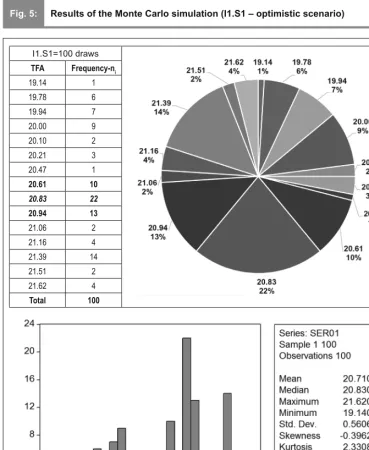
The analysis of the value of the variables described by a probability distribution was conducted statistically on several types of samples simulated by the Monte Carlo method (from 100 draws to 200; 300; 400; and fi nally 500 and 1,000 draws). In Fig. 5 and 6 one can distinguish the results of I1 (hypothesis 1) in the three scenarios (optimistic, realistic and pessimistic). The first normally distributed series in the simulations done was selected, in accordance with the Jarque-Bera test, where for a signifi cance level α = 0.01, the J-B statistics, calculated with the software package EViews, imposed a limit value of 9.21 and a critical probability greater than the pre-set signifi cance threshold α.
The realistic and pessimistic scenarios of the hypothesis 1 identify values of the J-B test that validate the normal distribution of the samples extracted (5.979 according to the realistic scenario, and 8.734 according to the pessimistic scenario) and provide a different range of variation in the total amount of funds accessed (based on averages of 19.74 and 16.6, respectively, as well as the Std. dev. values of 0.53 and 0.44, respectively). Fig. 6 shows the structure of the samples (100 draws in I1.S2 and 200 draws in I2.S3) and their specifi c distributions, where the ranges vary signifi cantly.
The appearance or the graphical contour of the normalized Kernel distributions for the three scenarios are described in Fig. 7, confi rming the insuffi cient coverage of the fi rst hypothesis by the incipient tendency of abnormality derived from multiplications with modal valences.
The I2 hypothesis, where the ratio of the variables of the two variants was 5/4, generates normally distributed samples of 100 draws (Tab. 8) in all scenarios.
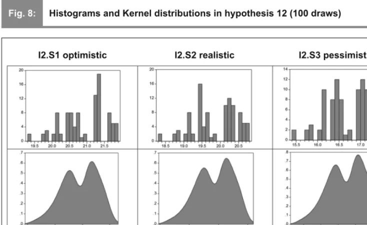
The histograms of the scenarios in hypothesis I2 and the normalized Kernel distributions describe a similar trend to abnormal distribution as in hypothesis I1 (Fig. 8).
With respect to hypothesis I3, with the same scenarios and samples of 500 draws, the simulations obtained were very close to the normal distribution as compared to the other hypotheses, i.e. I1 and I2, which failed to pass the J-B test, for samples larger than 200 and 400 draws, respectively. The optimal results as far as the Monte Carlo simulation in relation to
Sample 1 100 I2.S1. I2.S2. I3.S3.
Mean 20.906400 19.861400 16.725300
Median 21.050000 20.000000 16.840000
Maximum 21.850000 20.760000 17.480000
Minimum 19.360000 18.390000 15.490000
Std. Dev. 0.630253 0.598716 0.503034
Skewness -0.350413 -0.350238 -0.353759
Kurtosis 2.242042 2.246150 2.247688
Jarque-Bera 4.440237 4.412321 4.443974
Probability 0.108596 0.110123 0.108394
Source: made by the authors with the EViews package of programs
Tab. 8: Descriptive statistics of the three simulations using hypothesis I2
EM_3_2017.indd 27
28 2017, XX, 3
Fig. 5: Results of the Monte Carlo simulation (I1.S1 – optimistic scenario)
I1.S1=100 draws
TFA Frequency-ni
19.14 1
19.78 6
19.94 7
20.00 9
20.10 2
20.21 3
20.47 1
20.61 10
20.83 22
20.94 13
21.06 2
21.16 4
21.39 14
21.51 2
21.62 4
Total 100
Source: own Note:The sample of 100 normally distributed draws, arising from the application of the Monte Carlo method in keeping with the hypothesis I1.S1 (optimistic scenario). Software used Microsoft Excel and EViews.
EM_3_2017.indd 28
29 3, XX, 2017
Fig. 6: Results of the Monte Carlo simulation (I1.S2 – realistic and I1.S3 – pessimistic)
I1.S2 = 100 draws
TFA Frequency-ni
18.79 4
18.94 6
19.00 8
19.10 5
19.20 3
19.45 3
19.58 11
19.79 17
19.90 10
20.00 2
20.10 4
20.32 13
20.43 8
20.54 6
18.79 4
Total 100
1.S3 = 200 draws
TFA Frequency -ni
15.31 2
15.82 4
15.95 8
16.00 22
16.08 14
16.17 3
16.38 7
16.49 23
16.67 32
16.76 20
16.84 5
16.93 14
17.11 29
17.20 10
17.30 7
Total 200
Source: own Note:The make-up of the normally distributed samples of 200 and 100 draws, resulting from the application of the Monte Carlo method in keeping with hypotheses I1.S2 and I1.S3 (realistic and pessimistic scenarios). Software used Microsoft Excel and EViews.
EM_3_2017.indd 29
30 2017, XX, 3
the three hypotheses and scenarios are fully confi rmed by hypothesis I3: in samples of 1,000 draws all the three scenarios were distributed normally in keeping with the values of the J-B test and the normalized Kernel distribution, in parallel to I1 and I2 (Fig. 9).
The three scenarios of the Monte Carlo simulation, structured graphically, in the I3 hypothesis and in 1,000 draws samples, describe a much clearer and consistent prediction for each single case, which can be reduced to one or two defi ning values (Tab. 9).
In the fi rst fi nal interpretation, based on the Monte Carlo simulation, starting from the experience Romania had in the fi rst EU budget period, the optimistic prediction (Fig. 10) identifi es a value of the total funds or fi xed assets to be accessed of 21.1 billion euros (i.e. in the 21.0-21.2 interval), the realistic one – 20.0 billion euros (in the 19.9-20.1 interval), and the pessimistic one, in a context of marked instability, 16.9 billion euros (in the 16.8-17.0 interval).
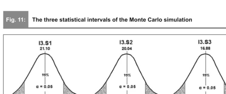
As the three scenarios stand the J-B test and thus identify normal distributions, in a rigorous statistical interpretation of prediction by means of the Monte Carlo simulation, three intervals are identifi ed within which the total amount will be placed of the European funds that will be accessed by Romania during the 2014-2020 period, with a signifi cance level
α = 0.05, or else guaranteed with a probability of 95 cases out of 100 (Fig. 11).
The concrete intervals of the Monte Carlo simulation for 1,000 draws, in keeping with hypothesis I3 and the three distinct scenarios, are detailed in Tab. 10.
The most likely of the intervals analyzed is, in the authors’ opinion, the one defi ned by the realistic hypothesis (I3S2 – the 1,000 draws sample).
Conclusions
The Monte Carlo simulation method has a predictive role, so it was preferred, in this paper, to the classical econometric type of modelling, as a solution to a complex problem of scenario and forecasting, in a context characterized by a high degree of uncertainty. This article transforms the classical predictions centred on mean values by means of the probabilistic thinking specifi c to the Monte Carlo method in simulations of random variables based on the inference of the estimators.
The Monte Carlo simulation also provides reliable solutions to identify and eliminate the internal ineffi ciencies of the process of accessing and absorbing EU funds. The main limitation of the simulation is related to the generation of hypotheses based solely on the experience in one budget cycle, completed by Romania in EU (faced with its average absorption rate), without however having a clearer algorithm of the cyclicality of the economic development specifi c to those areas. The authors are left with one chief concern for the perspective, namely identifying new hypotheses, scenarios and factorial or explanatory variables for EU funds absorption during the remaining period, 2017-2022, according to the n+2 principle of fi nal time assessing of European-funded projects.
Fig. 7: The normalized Kernel distributions for hypothesis I1 (100 and 200 draws)
Source: made by the authors with the EViews package of programs
EM_3_2017.indd 30
31 3, XX, 2017
Fig. 8: Histograms and Kernel distributions in hypothesis 12 (100 draws)
I2.S1 optimistic I2.S2 realistic I2.S3 pessimistic
Source: made by the authors with the EViews package of programs
Fig. 9: The normalized Kernel distributions in hypothesis I3 (1,000 draws)
I3.S1 optimistic I3.S2 realistic I3.S3 pessimistic
Source: made by the authors with the EViews package of programs
EM_3_2017.indd 31
32 2017, XX, 3
Fig. 10: The Monte Carlo simulation for hypothesis I3 (1,000 draws)
I3.S1 optimistic – 1,000 draws I3.S2 realistic – 1,000 draws
I3.S3 optimistic – 1,000 draws
Source: made by the authors with the Microsoft Excel package of programs
Sample: 1 1000 I3.S1 I3.S2 I3.S3
Mean 21.095440 20.040790 16.876450
Median 21.090000 20.040000 16.880000
Maximum 21.450000 20.380000 17.160000
Minimum 20.690000 19.660000 16.550000
Std. Dev. 0.131235 0.124620 0.104986
Skewness -0.052231 -0.049808 -0.049685
Kurtosis 2.888828 2.902035 2.906901
Jarque-Bera 0.969638 0.813361 0.772579
Probability 0.615809 0.665857 0.679574
Source: made by the authors with the EViews package of programs
Tab. 9: Descriptive statistics for hypotheis I3 – S1, S2, S3 (1,000 draws)
EM_3_2017.indd 32
33 3, XX, 2017
References
Benninga, S. (2008). Financial Modelling (3rd ed.). Cambridge, Massachusetts: MIT Press.
Burtescu, E. (2010). Sisteme informatice în afaceri. Craiova: Editura Sitech.
Creal, D. D. (2012). A survey of sequential Monte Carlo methods for economics and
fi nance. Econometric Reviews, 31(3), 245-296. doi:10.1080/07474938.2011.607333.
Del Moral, P., Doucet, A., & Jasra, A. (2006). Sequential Monte Carlo sampler. Journal of the Royal Statistical Society, Series B, 68(3), 1-26. doi:10.1111/j.1467-9868.2006.00553.x.
Dinu, V., Săvoiu, G., & Dabija, D.- C. (2016). A concepe, a redacta și a publica un articol științifi c. O abordare în contextul cercetării economice. București: Editura ASE.
Dobrescu, E. (2015). BARS curve in Romanian economy. Amfi teatru Economic, 17(39), 693-705.
Glasserman, P. (2004). Monte Carlo methods in fi nancial engineering. New York, NY: Springer. doi:10.1007/978-0-387-21617-1.
Jackel, P. (2002). Monte Carlo methods in
finance. New York: John Wiley and Sons. Kottemann, E. J. (2017). Illuminating Statistical Analysis Using Scenarios and Simulations. New Jersey, NJ: John Wiley & Sons, Inc. doi:10.1002/9781119296386.
Krivokapić, J., & Jaško, O. (2015). Global Indicators Analysis and Consultancy Experience Insights into Correlation Between Entrepreneurial Activities and Business Environment. Amfiteatru Economic, 17(38), 291-307.
Kucharavy, D., & De Guio, R. (2005). Problems of Forecast. ETRIA TRIZ Future Conference, 1, 219-235, Retrieved April 7, 2017, from https://hal.archives-ouvertes.fr/hal-00282761/document.
Kucharavy, D., & De Guio, R. (2012). Application of Logistic Growth Curve. In C. V. Machado, & H. V. Navas (Eds.), TRIZ Future Conference 2012 (pp. 41-53). Lisbon: Universidade Nova de Lisboa.
Maverick, J. B. (2016). What’ s the difference between a financial plan and a fi nancial
Scenario (α = 0.05) Mean ± 1.96 × Std.dev. Observations
S1 – optimistic [20.84 – 21.36] J-B = 0.97 and Std. dev. = 0.131
S2 – realistic [19.80 – 20.29] J-B = 0.81 and Std. dev. = 0.125
S3 – pessimistic [16.67 – 17.09] J-B = 0.77 and Std. dev. = 0.105
Source: own
Tab. 10: Real statistical intervals of values simulated with the Monte Carlo method in I3
Fig. 11: The three statistical intervals of the Monte Carlo simulation
Source: Graph drawn by the authors based on the data of the simulations in hypothesis S3
EM_3_2017.indd 33
34 2017, XX, 3
forecast? Retrieved March 1, 2017, from http:// www.investopedia.com/ask/answers/051315/ whats-difference-between-fi
nancial-plan-and-fi nancial-forecast.asp.
Mun, J. (2006). Modeling Risk: Applying Monte Carlo Simulation, Real Options Analysis, Forecasting, and Optimization Techniques (Wiley Finance). Hoboken, NJ: John Wiley & Sons, Inc. doi:10.1002/9781118366332.
Consiliul fi scal. (2015). Raport anual fi scal. Retrieved April 17, 2017, from http://www. consiliulfi scal.ro/RaportanualCF2015.pdf.
Robert, C. P., & Casella, G. (2004). Monte Carlo Statistical Methods (2nd ed.). New York, NY: Springer Press. doi:10.1007/978-1-4757-4145-2.
Săvoiu, G. (2007). Statistica - Un mod ştiinţific de gândire. București: Editura Universitară.
Săvoiu, G. (2013). Modelarea Economico-Financiară: Gândirea econometrică aplicată în domeniul fi nanciar. Bucureşti: Editura Universitară.
Săvoiu, G. (2016). European Integration through Economic Convergence. Amfi teatru Economic, 18(42), 237-238.
Săvoiu, G., Dima, F., Ene, S., Marcu, N., & Mihailov, L. (2006). Proiecte cu fi nanțare externă. Piteşti: Editura Independența Economică.
Săvoiu, G., Tudoroiu, L., & Burtescu, E. (2017). Using the Monte Carlo method to estimate the European funds absorbed by the Romanian economy from the EU in 2007-2013.
Romanian Statistical Review, Supplement 3, 110-119.
Simulation. (2012). In Encyclopaedia Britannica Online. Retrieved May 1, 2017, from https://www.britannica.com/science/simulation.
Țarțavulea (Dieaconescu), R. I., Belu, M. G., Paraschiv, D. M., & Popa, I. (2016). Spatial Model for Determining the Optimum Placement of Logistics Centers in a Predefi ned Economic Area. Amfi teatru Economic, 18(43), 707-725.
Prof. habil. Gheorghe Săvoiu, Ph.D. University of Pitesti Faculty of Economic Sciences and Law gheorghe.savoiu@upit.ro Assoc. Prof. Emil Burtescu, PhD University of Pitesti Faculty of Economic Sciences and Law emil.burtescu@yahoo.com
Prof. Vasile Dinu, PhD The Bucharest Academy of Economic Studies The Faculty of Business and Tourism dinu_cbz@yahoo.com
Ec. Ligian Tudoroiu, PhD Candidate S.C. Ronera SA Bascov and University of Craiova
l.tudoroiu@ronera.ro
EM_3_2017.indd 34
35 3, XX, 2017
Abstract
A MONTE CARLO METHOD SIMULATION OF THE EUROPEAN FUNDS THAT
CAN BE ACCESSED BY ROMANIA IN 2014-2020
Gheorghe Săvoiu, Emil Burtescu, Vasile Dinu, Ligian Tudoroiu
The authors dealt with fi nding some relevant simulation solutions for the value of the European funds that can be accessed by Romania in the second budget cycle (2014-2020) of the European Union (EU), in which the national economy is participating after the 2007 accession. The article presents, in a brief conceptual introduction, the option for simulation, not only as economical and statistical alternative but also as conceptual and technical method, followed by an analysis section for the EU funds accessed by Romania in the 2007-2013 fi nancial period and in the fi rst three years of 2014-2020 fi nancial period, with a role in generating hypotheses and scenarios of a type of modelling the process of accessing and specifi c absorption (including all types of rates, from the current absorption rate to the actual rate, with revenue in advance, etc.). A methodology section describes the rationale for selecting the method of simulation as Monte Carlo, and also the main hypotheses, detailed scenarios and integrated characteristic variables. The scenario-making eventually shaped three options by combining criteria of stability/instability, nuanced by optimistic/ pessimistic type scenarios. The analysis of the variables described by a probability distribution was conducted statistically on several types of samples simulated by the Monte Carlo method, from 100 draws to 200; 300; 400; and fi nally 500 and 1,000 draws.A presentation of the fi nal simulation results and a number of major comments regarding their calibration, confrontation, clarity and statistical analysis, together with some fi nal remarks as conclusions, limitations and perspectives, end the research approach.
Key Words: Simulation, Monte Carlo, European funds earmarked, EU funds accessed, the current absorption rate and the actual rate, revenue (in advance).
JEL Classifi cation: C53, C63, E17, E27, E37, F37, F47, G17.
DOI: 10.15240/tul/001/2017-3-002
EM_3_2017.indd 35