Learn to Human-level Control in Dynamic Environment
Using Incremental Batch Interrupting Temporal
Abstraction
Yuchen Fu1, Zhipeng Xu1, Fei Zhu1,2,3,4, Quan Liu1,3, and Xiaoke Zhou5 1
School of Computer Science and Technology, Soochow University, Shizi Street No.1 Box 158, Suzhou, China, 215006
[email protected], [email protected],
{zhufei, quanliu}@suda.edu.cn
2 Provincial Key Laboratory for Computer Information Processing Technology Soochow University
3 Collaborative Innovation Center of Novel Software Technology and Industrialization 4
Key Laboratory of Symbolic Computation and Knowledge Engineering of Ministry of Education, Jilin University, Changchun, 130012, P.R. China
5
University of Basque Country, Spanish [email protected]
Abstract. The temporal world is characterized by dynamic and variance. A lot of machine learning algorithms are difficult to be applied to practical control applica-tions directly, while hierarchical reinforcement learning can be used to deal with them. Meanwhile, it is a commonplace to have some partial solutions available, called options, which are learned from knowledge or predefined by the system, to solve sub-tasks of the problem. The option can be reused for policy determination in control. Many traditional semi-Markov decision process methods take advantage of it. But most of them treat the option as a primitive object. However, due to the uncertainty and variability of the environment, they are unable to deal with real world control problems effectively. Based on the idea of interrupting option under the prerequisite for dynamic environment, a Q-learning control method which uses temporal abstraction, named as I-QOption, is introduced. The I-QOption approach combines the idea of interruption with the characteristics of dynamic environment so as to be able to learn and improve control policy in dynamic environment. The Q-learning framework helps to learn from interaction with raw data and achieving human-level control. The I-QOption algorithm is applied to grid world, a bench-mark dynamic environment evaluation testing. The experiment results show that the proposed algorithm can learn and improve policy effectively in dynamic envi-ronment.
Keywords:hierarchical reinforcement learning, option, reinforcement learning, on-line learning, dynamic environment.
1.
Introduction
of generalization. The reinforcement learning algorithm take advantage of reinforcement learning agent to constantly interact with the unknown environment during the process of solving the problem [2],[31]. As an important algorithm of reinforcement learning, the temporal difference (TD) learning is capable of learning directly from raw experience without determining dynamic model of environment in advance. Moreover, the model learned by temporal difference is updated by estimation which is based on part of learn-ing rather than final results of the learnlearn-ing. TD learnlearn-ing is particularly suitable for solvlearn-ing the prediction problems and control problems in real-time control applications. The Q-learning, which is an off-policy version of TD Q-learning, is capable of reducing the com-putational complex, and achieving human-level control.
However, as the scale of the problem to be solved gets larger and larger, the rein-forcement learning agent requires more and more time, computation and information to learning and make decisions. As a result,the agent usually fails to work because it cannot handle mountains of data efficiently [14],[29]. Therefore, it seems to be essential to learn knowledge by interacting with the environment so as to attain a better policy for temporal decision making [20],[28]. As it has been revealed that the world is organized by some structures which contain information to help to make decision, we anticipate that the agent requires less computation by fully taking advantage of the structure of environment [13]. Botvinick et al. uses hierarchical reinforcement learning to make decisions [4]. Further-more, the hierarchical reinforcement learning methods proposed by Bakker et al. made use of sub-goal discovery and sub policy specialization [1]. More recently, Jardim et al. [10] extended the abstraction to state and then put forward an algorithm to learn sub-goals and sub-states in the hierarchical reinforcement learning. The option frameworks reviewed by Barto et al. [3], which were based on temporal abstraction proposed by Sutton et al. [27], have been used in many systems. Although options provides a very useful frame-work for temporal abstraction, most frame-work used sub-task to represent options [30],[11], correspondingly, many work aimed to find the sub-tasks [7]. For example, McGovern et al. used diverse density to automatically find sub-goals of reinforcement learning tasks [17]. Menache et al. put forward a Q-cut-dynamic method to discovery sub-goals [18]; S¸ims¸ek et al. introduced a method which used relative novelty to identify useful temporal abstraction [23] and a method which utilized local graph partitioning [24]. There are also lots of other work to extract options such as the value function [6], bisimulation metrics [5], visit frequency [26], via clustering[16], Using Ant System [8] and graph theory based method [12],[22].
An available temporal abstraction option is very critical to solve the problem effi-ciently [19]. The work [28] have had a preliminary study on it. However, his research was based on the setting of an ordinary simple condition, and therefore can not be applied in the real dynamic environment. Hence, in this work, we introduce the idea of interrupting to solve learning and controlling problems in dynamic environments, which brings two advantages: extending the ability of agent to solve the problems by introducing the idea of interrupting, which traditional option-based methods cannot deal with, and reducing the efforts by using SMDP methods.
2.
Related Work
2.1. Reinforcement Learning
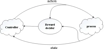
Reinforcement learning is a kind of machine learning method by interacting with the environment and mapping the states to the actions. In reinforcement learning, the agent evaluates the quality of actions by reward function and then takes the action that brings about the maximum returns, and thus the action will not only affect the immediate reward but also affect the reward of the next step, which is also known as reward of the next state [15]. Trial and error search as well as delayed reward are the important features of reinforcement learning. The reinforcement learning framework has five fundamental ele-ments: controller, environment, state, reward, and action, showed as Fig. 1. The controller, which learns knowledge by interacting with outside environment and then chooses an ac-tion in accordance with the decision made by established controlling model, is the agent of the system; accordingly, the state will then be changed; the environment will return a reward for evaluating. Most of reinforcement learning methods are based on Markov
De-Fig. 1.The Framework of reinforcement learning.
cision Process (MDP) which is represented by a tuple< X, U, f, ρ, γ >, whereX andU respectively represent a finite set of states and a set of actions,f ∈[0,1]represents tran-sition probability,ρ:X×U → ℜdenotes the rewards received by agent, andγ∈[0,1] represents discounted factor. At each time step, agent observes system statex∈X then takes an action, and then the state of the system transfers to next state x′ ∈ X with probabilityf(x, u, x′), and agent will get an immediate reward. The goal of the agent is to find the optimal policyh∗:X×U →[0,1]through maximizing the cumulative expected reward [25].
At each time stept, the agent selects an actionut ∈ U from action spaceU. As a result, the state of the system transfers toxt+1 ∈ X fromxt∈ Xin accordance with a function of transition probabilityf(xt, ut, xt+1):
xt+1=f(xt, ut) (1)
The agent attains a rewardrt+1according to rewarding functionρ:
The state-action value functionQh:X×U → ℜunder policyhis denoted as follows:
Qh(x, u) =
∞ ∑
t=0
γtρ(xt, ut) (3)
whereγ∈[0,1]is a discount rate which shows how far sighted the agent is in considering the rewards and is also a factor for increasing uncertainty on future rewards.
TD is capable of learning directly from raw experience without determining dynamic model of environment in advance. Moreover, the model learned by temporal difference is updated by estimation which is based on part of learning rather than final results. These two characteristics of TD make it particularly suitable for solving the prediction and con-trol problems in real-time concon-trol applications. Given some experience with policy h, temporal difference learning updates estimated V-value function as:
V(xt)←V(xt) +α[Rt−V(xt)] (4) whereRtis actual return after time stept,αis a step size parameter. TD estimatesV(t) in stept+ 1using the observed rewardrt+1.
LetQh(x, u)be the value of taking actionu∈Uunder a policyh.Qh(x, u)is defined as:
Qh(x, u) =ρ(x, u) +
∞ ∑
k=1
γkρ(xk, uk) (5)
Q-learning is an off-policy version of TD method, which is defined by:
Q(xt, ut)←Q(xt, ut) +α[rt+1+γmax
u Q(xt+1, u)−Q(xt, ut)] (6) The ultimate goal of reinforcement learning agent is to get an optimal policyh∗. The corresponding optimal value functionV∗(x)and state-action value functionQ∗(x, u)can be represented as:
V∗(x) = max
u∈U{ρ(x, u) +γ
∑
x∈X
f(x, u, x′)V∗(x′)} (7)
Q∗(x, u) =ρ(x, u) +γ∑ x∈X
f(x, u, x′) max u∈UQ
∗(x′, u′) (8)
2.2. Options
In this work, we use Markov option [31] to represent the terms of temporal abstraction. Temporal abstractions and primitive actions are both actions selected by the agent. During the execution of an option, agent takes policyhof the option until the terminal condition of the option is satisfied. Generally, an option can be modeled by a triplet< I, h, β >. The input set of option is expressed byI,I ∈X, which means an option< I, h, β >is available atx∈I. Policyh:X×U →[0,1]denotes the internal policy ofoand terminal conditionβ :X →[0,1].
ut←h(xt); and the state of the system will transfer toxt+1, namely(xt, h) ut
−→xt+1. Agent will determine whether to end the execution ofoatxt+1according to the termi-nal conditionβ. If the execution is not interrupted,owill continue to be executed until a terminal conditionβ(xt+k) → 1is satisfied. So there existsβ(x) → 0for all primi-tive actions. When an option terminates, agent could choose another option or choose a primitive action. We will use an example to illustrate option. A robot is required to open a door. The whole process is composed of inserting the key, holding the lock, rotating the lock, and opening the door. If we use the concept of option, the process can be regarded as an action sequence: inserting the key, holding the lock, and rotating the lock. During this process, agent standing by the door can starts with an initial state of optiono. The next action executed by the agent could be inserting the key according theo’s policy and then get to the next state recursively. The terminal state of the system should be that rotating the lock andois terminated at the time. Consequently the agent will then select the next option or primitive action. In fact, the option also includes primitives actions, where all the primitive actions meetβ(x)→0.
Now we can define policy on option. Let the available option set beOxatxt, when the agent starts from statext, an optionowill be chosen with probability ofv(xt, o), where o∈Oxandvis a Markov policy. Then actions will be selected according to policyhof optionountilois terminated at statext+kafter k steps; and then the next optiono′will be selected accordingv(xt+k). Actually, the policyv defined over optionodetermined the flat policyydefined on primitive actions, and we can gety=f(v). So we can define the value of a state under the flat policy at statext:
Vy(xt) =E{rt+1+γrt+2+γ2rt+3+· · · |ε(y, xt, t)} (9) whereε(y, xt, t)denotes the history that agent start from statextat timetunder policy y. Due to this formula is based on the primitive actions, but policyyis determined byv, so there existVy(xt) =Vf(v)(xt). Similarly we can get:
Qv(xt, o) =E{rt+1+γrt+2+γ2rt+3+· · · |ε(vo, xt, t)} (10) whereε(yo, xt, t)denotes the process that agent select optionofirst under policyvuntil ois terminated and select other options.
2.3. Semi-Markov Decision Problems (SMDPs)
A reinforcement learning task which satisfies the Markov property is considered as Markov decision processes (MDPs). We believe that a semi-Markov Decision Process (SMDP) can be constituted by any MDP and a fixed set of options [27]. Cnventional SMDP theory is associated with the actions and related methods can be extended to options [21]. Thus, for any optiono, ifε(o, xt, t)denotes the process thatostarts from statextat timet, then the corresponding reward model will be:
ρ(xt, o) =E{rt+1+γrt+2+γ2rt+3+· · ·+γk−1rt+k|ε(o, xt, t)} (11) wheret+krepresent termination time of optiono. Similarly, the transition probability model will be defined as follows:
f(xt, o, xt+k) =
∞ ∑
k=1
wheref(xt+k, k) denotes the probability thato terminates after k steps at statext+k. Then according to Bellman equation, for any Markov policyh, the state value function can be defined as:
Vh(xt) =
∑
o∈Oxth(xt, o)[ρ(xt, o) +
∑
xt+k
f(xt, o, xt+k)Vu(xt+k)] (13) Corresponding state-action value function can be defined as:
Qh(xt, o) =ρ(xt, o) +
∑
xt+k
f(xt, o, xt+k)Vh(xt+k) (14) On the basis of the value function, we can get the optimal value function. In MDPs, we select optimal action, correspondingly, we select optimal option. We denote options set byOhere. According to Bellman optimal equation, we can obtain the optimal state value function:
V∗(xt) = maxo∈Oxtρ(xt, o) +
∑
xt+k
f(xt, o, xt+k)V∗(xt+k) (15) And the optimal state-action value functions:
Q∗(x, o) =ρ(xt, o) +
∑
xt+k
f(xt, o, xt+k)V∗(xt+k) =ρ(xt, o) +
∑
xt+k
f(xt, o, xt+k)maxo′∈Oxt
+kQ
∗(x
t+k, o′)
(16)
According to the optimal value function, we can get updating formula ofQ:
Qh(xt, o)←Qh(xt, o) +α[ρ(xt, o) +γkmax o′ Q
h(x
t+k, o′)−Qh(xt, o)] (17) If the option set has already been obtained, then we can compute the optimal state value function and the optimal action value function. Finally we can obtain the optimal pol-icy through interacting with the environment. Moreover, the standard SMDP theory can guarantee that such process can converge.
3.
Algorithm description
3.1. Interrupting Option
3.2. Incremental Batch Updating Approach
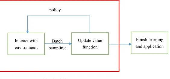
Batch reinforcement learning is often used to describe a set of reinforcement learning that complete learning from a group of samples, the key lies in batch mode algorithm is the way it processes a batch of sample and gets the best results from it. The benefits of batch updating are the stability of the learning process and the validity of the data, and reinforcement learning methods using batch updating usually converge faster to a certain extent. By using batch reinforcement learning all of the observed transition samples are stored and synchronous updating on the entire sample. However, if it is in accordance with the first storing all the samples and then updating to learn a good policy, policy of reinforcement learning agent will not be updated during sampling. In practice, sampling has a great influence on the quality of policy. At the same time, the samples for reinforce-ment learning agent must be similar to the actual transition sample of the system in order to get a good policy. The simplest way to solve it is to interact with the system to sample, which gives rise to incremental batch updating methods between online learning methods and batch updating methods. The process of incremental reinforcement learning methods for batch updating learning is shown in Fig. 2.
policy
Interact with
environment
Update value
function Batch
sampling
Finish learning
and application
Incremental batch reinforcement
learning process
Fig. 2.The process of incremental batch reinforcement learning methods.
3.3. Algorithm I-QOption
finished without any termination halfway. As a matter of fact, this approach is known to be confronted with the problem in both cases. Firstly, the efficiency will be very poor in a dynamic environment as usually the option has been stalled before it ends as planned; secondly during the execution of the option, in certain states, it would be better to select another option. In this case, our algorithm should be applied to interrupt current option at appropriate time.
Suppose we’ve got the value function of an option under policyh, wherehis a global policy and(x, o)is a state option pair. The state-option value functionQh(x, o)cannot only evaluate the quality of current policyh, but also evaluate the quality of every step we take. Assume that at time step t, according to policyh, agent has selected optiono, then we can compare the value that agent executeowith the value that interruptoand select new option:
Vh(x) =∑ o′u(x, o
′)Qh(x, o′)
IfVh(xt)> Qh(xt, o)orQh(xt, ot)< Qh(xt+1, ot)whenxt+1=xt, we will interrupt oand complete an incremental batch updating, and then select another option to continue. The description of the algorithm is given as follows.
Algorithm 1I-QOption
Require: discounted factorγ, learning rateα, option setOg
1: InitializeQ(x, o)arbitrarily,whereo∈O
2: repeat
3: Initializext
4: repeat
5: Select an optiono(according to the initial exploration strategyh) 6: Execute optiono
7: repeat
8: Select actionu(according toho(xt))
9: Observe next state and rewardxt+1, r 10: Savext, xt+1, r
11: xt←xt+1
12: if Qh(xt, ot) < Qh(xt+1, ot) when xt+1 = xt or Vh(xt) > Qh(xt, o) or
β(xt+1) = 1then
13: Batch updatingQh(xt, o)for everyxtino
14: β(xt+1) = 1
15: end if
16: untiloended
17: Select new optiono′according toQ(xt, o)
18: untilxt+1is the terminal state 19: untilconvergence
3.4. Algorithm Analysis
Definition 1. For any MDP, any option setOand arbitrary Markov policyh, we define
denote a correspondingo′ ∈ O for everyo =< I, ho, β >∈ O, whereβ =β′ except Qh(h
o, o)< Vh(x),H represents history andxrepresents the last state of historyH.
We will terminateo′ at statex, namelyβ′(x) = 1. All of the history interrupt like this is
called interrupting history.
Theorem 1. Let h′ over o′ to be the corresponding policy of h : h(x, o) = h′(x, o′),
then: 1.Vh′(x) ≥Vh(x)for allx ∈ X; 2.there is a non-zero probability to encounter
interrupting history if initialized from state x ∈ X, then there is Vh′(x) > Vh(x);
3.limk→∞Vk(x) =Vo∗(x)for all ofx∈X, o∈O, that is the algorithm can converge to
a fixed point.
Proof. The idea is to execute improved policyh′by improving its terminal condition for
any statex, that is, we need to prove that the following inequality is satisfied
∑
o′h
′(x, o′)[ρ(x, o′) +∑
x′f(x, o
′, x′)Vh
(x′)]≥Vh(x) (18)
whereVh(x) =∑oh(x, o)[ρ(x, o) +∑x′f(x, o′, x′)Vh(x′)], if inequality (18) is
satis-fied, we can use it to extend the left part by using
∑
o′h
′(x, o′)[ρ(x, o′) +∑
x′f(x, o
′, x′)Vh(x′)]
constantly. In the limit case, the left formula turns to beVh. Then we can getVh′ ≥Vh. Because ofh′(x, o′) =h(x, o),∀x∈X, we need to proof :
ρ(x, o′) +∑ x′f(x, o
′, x′)Vu(s′)≥ρ(x, o) +∑
x′f(x, o, x
′)Vh(x′) (19)
LetΦdenote all the interrupting historyΦ={H ∈Ω : β(H) ̸=β′(H)}, then the left side of inequality (19) can be rewritten as:
E{r+γkVh(x′)|ϵ(o′, x), Hxx′ ∈/ Φ}+E{r+γkVh(x′)|ϵ(o′, x), Hxx′∈Φ} (20) wherex′denotes the next state,rdenotes the immediate reward andkdenotes step num-ber after following optionofrom state xrespectively. The history from statextox′ is denoted byx′. Due to encounter the trajectoryHxx′ ∈/ Φ, so the trajectory will be ter-minated, and it will be occur with the same probability and expectation after executeoat statex. Therefore, the right side of the inequality (19) can be rewritten as:
E{r+γkVh(x′)|ϵ(o′, x), Hxx′ ∈/ Φ}+ E{β(x′)[r+γkVh(x′)] + (1−β(x′))[r+ γkQh(Hxx′, o)]|ϵ(o′, x), hxx′ ∈Φ}
(21)
BecauseQh
4.
Experiment and Results
As the uncertainty of the environment in the real world, conventional SMDP methods ap-plied to options cannot be utilized efficiently, we use the option in a dynamic environment here to solve the task better. We will use the famous gridworld simulation experiment to evaluate the behaviour of I-QOption compared with Q-learning, and then we will give the experimental results below.
In the simulation experiment, agent uses theε−greedypolicy to complete explo-ration, the initial exploration probability is set to be ε = 0.1 and the learning rate is set to be α = 0.1. In order to let the algorithm to get a better convergence, the explo-ration probability will decay with the increase of the number of the episode. Here we set ε←ε/episode. All of theQvalue will be initialized to 0.
4.1. Dynamic Environment Description
So far, most of the reinforcement learning methods are applied to some simple learning task or learning in a static environment, such as balancing pole, DC motor, roller coaster, etc. However, real-world environment is usually not static. For example, in the room nav-igation task, there is no obstacle besides wall in general environment, even if there are obstacles, the position of those obstacles will not change over time. In real-world room navigation task, the random appearance of obstacles are very normal. Our target is to find optimal policy in a dynamic, ever-changing environment.
Fig. 3 gives an example of dynamic environment, it is a grid of21×21. There are two kinds of objects in this environment: agent and obstacles. The uppercase letter o in the left lattice in Fig. 3(a) indicates the position of the obstacle at episodetwhile the letter o in the right lattice in Fig. 3(b) indicates the position of the obstacle in episodet+k. As can be seen that in a different episode the location of the obstacle may not be the same.
S
O
G
(a)
S
O
G
(b)
4.2. Four-Room Dynamic Gridworld
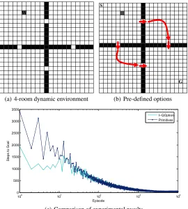
We give a four-room dynamic gridworld environment shown in Fig. 4(a). The goal state Gis placed in the lower right corner and the initial state S is placed in the upper left corner. At the beginning of each episode, we will provide random obstacles, besides the fixed obstacles, to represent the random environment. The primitive action consists of four direction actions: up, down, left and right. The selection probability of greedy action (primitive action or option) is1−ε+ε/(|U|x+|O|x), and the selection probability of other action or option isε/(|U|x+|O|x). The reward is set to be -1 except the step to the goal state which has been set to be 1.
W
(a) 4-room dynamic environment
S
G
(b) Pre-defined options
100 101 102 103 104
0 500 1000 1500 2000 2500 3000 3500
Episode
St
e
p
s
to
G
o
a
l
I−QOption Primitives
(c) Comparison of experimental results
Fig. 4.Comparison of I-QOption algorithm and Q-learning in four-room dynamic envi-ronment.
Since the focus of this paper is the application of option in dynamic environments, therefore, the options here are predefined. We provide six options as prior knowledge in the four-room gridworld shown in 4(b).
Q-learning in the dynamic gridworld. As can be seen from Fig. 4(c), the step I-QOption needs to reach the goal state is far less than Q-learning in the first few episodes. In the first episode I-QOption needs only 1829 steps while Q-learning needs 2542 steps. The Fig. 4(c) also shows that the convergence rate of I-QOption is slightly faster than Q-learning. I-QOption converges at the episode 3708 while Q-learning converges at episode 3787.
As can be seen from Fig. 4(c), in the four-room dynamic environment, the perfor-mance of I-QOption is significantly better than Q-learning which based on primitive ac-tions in the first few episodes, and this phenomenon is particularly evident in the first 10 episodes. After 10 episodes, the performance of I-QOption and Q-learning is roughly equal, but I-QOption still has a faster convergence rate than Q-learning for about 80 episodes. The simulation results indicate the effectiveness of the algorithm in dynamic environments.
4.3. Six-Room Dynamic Gridworld
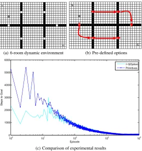
In the second experiment described in this paper, we use six-room dynamic gridworld to simulate experiments. The task of the agent is the same as that of four-room dynamic gridworld. Fig. 5(a) shows the experimental environment, the initial state close to the upper left corner while the goal state near the lower right corner. Dynamic environment and primitive actions are set to be the same as introduced before.
As described in the previous section, the number of option pre-defined here will be a corresponding increase due to the number of room increased. In the six-room experiment, 10 options will be pre-defined while six options are provided in the four-room experiment as Fig. 5(b) shown. Fig. 5(c) shows the average step number that agent from the start state to reach the goal state, based on 10 repeated experiments. The difference with Fig. 4(c) is that the number of steps that agent needs to reach the goal state at early moment has increased due to the increasing of the state number. At the same time, the convergence rate also has slowed down, but the trend is the same overall.
We can draw the similar conclusion with the experiment results in the previous sec-tion, in the early stages of learning, I-QOption is much better than Q-learning, and in the latter study, the convergence rate of I-QOption is slightly better than Q-learning.
4.4. Results by Different Parameters Settings
There are three parameters in our algorithm: step size α, exploring probability ε, and discounted factorγ, whereεandγusually have a general value, such asε= 0.1.
G S
(a) 6-room dynamic environment
S
G
(b) Pre-defined options
100 101 102 103 104
0 1000 2000 3000 4000 5000 6000
Episode
St
e
p
s
to
G
o
a
l
I−QOption Primitives
(c) Comparison of experimental results
Fig. 5.Comparison of I-QOption algorithm and Q-learning in six-room dynamic environ-ment.
In the case of learning rate a = 0.9, I-QOption only requires 1687 time steps to reach goal in the first episode, while Q-learning needes 2995 time steps. The results suggest that we can accelerate the convergence by increasing the learning rate when the rate is within the acceptable range.
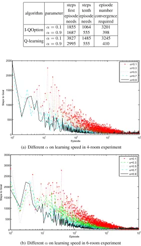
As can be seen from Fig. 6, both in the four-room and six-room experiments, the effects of different values of the algorithm are great. We can conclude that the learning speed of the agent has accelerated with the increase ofα. Agent learns faster than other parameter values when α = 0.9, and the performance is better in the learning phase. The proposed algorithm converges in the eightieth episode and maintain stability when α= 0.9.
Table 1.Comparison of I-QOption algorithm and Q-learning with different parameters in the 4-room experiment.
algorithm parameter steps first episode needs steps tenth episode needs episode number convergence required I-QOption α= 0.1 1855 1064 3201
α= 0.9 1687 555 398
Q-learning α= 0.1 3827 1485 3245
α= 0.9 2995 555 410
100 101 102 103 104
0 500 1000 1500 2000 2500 Episode St e p s to G o a l α=0.1 α=0.3 α=0.5 α=0.7 α=0.9
(a) Differentαon learning speed in 4-room experiment
100 101 102 103 104
0 500 1000 1500 2000 2500 3000 3500 Episode St e p s to G o a l α=0.1 α=0.3 α=0.5 α=0.7 α=0.9
(b) Differentαon learning speed in 6-room experiment
the earlier learning phase, the value ofQ(x, u)with a large value ofαtends to update quickly, which leads to the algorithm convergence in a short period of time. But because of the exploration of our algorithm, after the convergence of the algorithm, the large value ofαleads to a more updating on exploration actions, which will causes larger fluctuation range.
5.
Conclusions
Reinforcement learning enables to learn and optimize control from the interaction with environment. It is flexible and can be applied in many different applications. As a fa-mous algorithm of reinforcement learning, Q-learning is able to learn directly from raw experience like human and does not need to know the environment model in advance.
In this work we introduce interrupting mechanism to SMDP option on the basis of Q-learning to address dynamic environments. The algorithm, called interrupting Q-Q-learning option, is able to better solve the problem in a dynamic environment which traditional op-tion based methods are unable to deal with. The experiment results show that the appro-priate use of interrupting option can accelerate solving tasks in a dynamic environment, and also it will be help for agent to keep stability during the process of learning.
Acknowledgments.This paper is supported by National Natural Science Foundation of China (61303108, 61373094, 61472262), High School Natural Foundation of Jiangsu(13KJB520020), Key Laboratory of Symbolic Computation and Knowledge Engineering of Ministry of Educa-tion, Jilin University(93K172014K04), Suzhou Industrial application of basic research program part (SYG201422), Provincial Key Laboratory for Computer Information Processing Technology, Soochow University(KJS1524).
References
1. Bakker, B., Schmidhuber, J.: Hierarchical reinforcement learning based on subgoal discovery and subpolicy specialization. In: Proc. of the 8-th Conf. on Intelligent Autonomous Systems. pp. 438–445 (2004)
2. Barto, A.G.: Reinforcement learning: An introduction. MIT press (1998)
3. Barto, A.G., Mahadevan, S.: Recent advances in hierarchical reinforcement learning. Discrete Event Dynamic Systems 13(4), 341–379 (2003)
4. Botvinick, M.M.: Hierarchical reinforcement learning and decision making. Current opinion in neurobiology 22(6), 956–962 (2012)
5. Castro, P.S., Precup, D.: Automatic construction of temporally extended actions for mdps using bisimulation metrics. In: Recent Advances in Reinforcement Learning, pp. 140–152. Springer (2012)
6. Chaganty, A.T., Gaur, P., Ravindran, B.: Learning in a small world. In: Proceedings of the 11th International Conference on Autonomous Agents and Multiagent Systems-Volume 1. pp. 391–397. International Foundation for Autonomous Agents and Multiagent Systems (2012) 7. Drummond, C.: Accelerating reinforcement learning by composing solutions of automatically
identified subtasks. Journal of Artificial Intelligence Research 16(1), 59–104 (2002)
8. Ghafoorian, M., Taghizadeh, N., Beigy, H.: Automatic abstraction in reinforcement learning using ant system algorithm. In: AAAI Spring Symposium: Lifelong Machine Learning (2013) 9. Girgin, S., Polat, F., Alhajj, R.: Improving reinforcement learning by using sequence trees.
10. Jardim, D., Nunes, L., Oliveira, S.: Hierarchical reinforcement learning: learning sub-goals and state-abstraction. In: Information Systems and Technologies (CISTI), 2011 6th Iberian Conference on. pp. 1–4. IEEE (2011)
11. Jin, Z., Jin, J., Liu, W.: Autonomous discovery of subgoals using acyclic state trajectories. In: Information Computing and Applications, pp. 49–56. Springer (2010)
12. Kazemitabar, S.J., Beigy, H.: Automatic discovery of subgoals in reinforcement learning using strongly connected components. In: Advances in Neuro-Information Processing, pp. 829–834. Springer (2008)
13. Konidaris, G., Barto, A.G.: Building portable options: Skill transfer in reinforcement learning. In: IJCAI. vol. 7, pp. 895–900 (2007)
14. Korf, R.E.: Macro-operators: A weak method for learning. Artificial intelligence 26(1), 35–77 (1985)
15. Lin, L.J.: Self-improving reactive agents based on reinforcement learning, planning and teach-ing. Machine learning 8(3-4), 293–321 (1992)
16. Mannor, S., Menache, I., Hoze, A., Klein, U.: Dynamic abstraction in reinforcement learning via clustering. In: Proceedings of the twenty-first international conference on Machine learning. p. 71. ACM (2004)
17. McGovern, A., Barto, A.G.: Automatic discovery of subgoals in reinforcement learning using diverse density. Computer Science Department Faculty Publication Series p. 8 (2001) 18. Menache, I., Mannor, S., Shimkin, N.: Q-cut-dynamic discovery of sub-goals in reinforcement
learning. In: Machine Learning: ECML 2002, pp. 295–306. Springer (2002)
19. Osentoski, S., Mahadevan, S.: Basis function construction for hierarchical reinforcement learn-ing. In: Proceedings of the 9th International Conference on Autonomous Agents and Multiagent Systems: volume 1-Volume 1. pp. 747–754. International Foundation for Autonomous Agents and Multiagent Systems (2010)
20. Precup, D.: Temporal abstraction in reinforcement learning (2000)
21. Precup, D., Sutton, R.S., Singh, S.: Multi-time models for temporally abstract planning. Ad-vances in neural information processing systems pp. 1050–1056 (1998)
22. S¸ims¸ek, ¨O., Barreto, A.S.: Skill characterization based on betweenness. In: Advances in neural information processing systems. pp. 1497–1504 (2009)
23. S¸ims¸ek, ¨O., Barto, A.G.: Using relative novelty to identify useful temporal abstractions in re-inforcement learning. In: Proceedings of the twenty-first international conference on Machine learning. p. 95. ACM (2004)
24. S¸ims¸ek, ¨O., Wolfe, A.P., Barto, A.G.: Identifying useful subgoals in reinforcement learning by local graph partitioning. In: Proceedings of the 22nd international conference on Machine learning. pp. 816–823. ACM (2005)
25. Singh, S., Jaakkola, T., Littman, M.L., Szepesv´ari, C.: Convergence results for single-step on-policy reinforcement-learning algorithms. Machine Learning 38(3), 287–308 (2000)
26. Stolle, M., Precup, D.: Learning options in reinforcement learning. In: Abstraction, Reformu-lation, and Approximation, pp. 212–223. Springer (2002)
27. Sutton, R.S., Precup, D., Singh, S.: Between mdps and semi-mdps: A framework for temporal abstraction in reinforcement learning. Artificial intelligence 112(1), 181–211 (1999)
28. Sutton, R.S., Singh, S., Precup, D., Ravindran, B.: Improved switching among temporally ab-stract actions. Advances in neural information processing systems pp. 1066–1072 (1999) 29. Szepesvari, C., Sutton, R.S., Modayil, J., Bhatnagar, S., et al.: Universal option models. In:
Advances in Neural Information Processing Systems. pp. 990–998 (2014)
30. Thrun, S., Schwartz, A., et al.: Finding structure in reinforcement learning. Advances in neural information processing systems pp. 385–392 (1995)
Yuchen Fuis a member of China Computer Federation. He is a PhD and professor. His research interest covers reinforcement learning, intelligence information processing, and deep Web.
Zhipeng Xuis a postgraduate student in the Soochow University.His main research in-terests include reinforcement learning and machine learning.
Fei Zhuis a member of China Computer Federation. He is a PhD and an associate pro-fessor. His main research interests include reinforcement learning, image processing, and pattern recognition. He is the corresponding author of this paper.
Quan Liu is a member of China Computer Federation. He is a PhD, post-doctor, pro-fessor and PhD supervisor. His main research interests include reinforcement learning, intelligence information processing and automated reasoning.
Xiaoke Zhouis now an assistant professor of University of Basque Country UPV/EHU, Faculty of Science and Technology, Campus Bizkaia, Spain. He majors in computer sci-ence and technology. His main interests include machine learning, artificial intelligsci-ence and bioinformatics.