EVAPORATION DEPTH CONTROLS THE RELATIONSHIP BETWEEN SOIL WATER MOBILITY AND SOIL WATER ISOTOPIC COMPOSITION
by
John Byars Shuler
A thesis
submitted in partial fulfillment of the requirements for the degree of Master of Science in Hydrologic Sciences
Boise State University
© 2018
DEFENSE COMMITTEE AND FINAL READING APPROVALS
of the thesis submitted by
John Byars Shuler
Thesis Title: Evaporation Depth Controls the Relationship Between Soil Water Mobility and Soil Water Isotopic Composition
Date of Final Oral Examination: 4 May 2018
The following individuals read and discussed the thesis submitted by student John Byars Shuler, and they evaluated his presentation and response to questions during the final oral examination. They found that the student passed the final oral examination.
James P. McNamara, Ph.D. Chair, Supervisory Committee
Shawn Benner, Ph.D. Member, Supervisory Committee
Matthew J. Kohn, Ph.D. Member, Supervisory Committee
iv
ACKNOWLEDGEMENTS
I would like to thank my Supervisory Committee chair, Dr. Jim McNamara, for his guidance during the completion of this thesis and his patience while I learned how to be a student again. I would also like to thank the members of my Supervisory Committee, Dr. Shawn Benner and Dr. Matt Kohn, for their invaluable input throughout the process. Without my committee’s expertise, this thesis would not have been possible. I owe additional gratitude to Dr. Kohn for access to his Stable Isotope Laboratory, where I spent many late hours processing samples.
Research Scientists Samantha Evans and Pam Aishlin provided endless assistance and advice in both the lab and field and I cannot thank them enough. The list of
individuals who gave their time to assist with field and lab work is too long to list here, but their selflessness and companionship was vital to the project and my sanity. The love and encouragement of my friends, family, and wife, Kathleen Pritchard, have been a steadying influence during my graduate school career and throughout my life.
v ABSTRACT
Recent studies of plant water uptake assume that soil water isotopic composition can be used to infer soil water mobility. However, the strength of the relationship
between mobility and isotopic composition remains poorly constrained. In addition, many ecohydrologic investigations are restricted by low sampling frequencies and insufficient soil moisture and matric potential data to support assumptions of soil water mobility. We sampled bulk soil water every 14 to 21 days in hillslope and riparian profiles during the 2016 and 2017 growing seasons in a semi-arid watershed outside Boise, ID. We collected twig samples of four tree and shrub species concurrently. Plant and soil water samples extracted by cryogenic vacuum distillation were analyzed for δ2H and δ18O composition. We installed volumetric water content and soil matric potential sensors at five and four depths in the hillslope profile, respectively. Shallow bulk soil water became progressively enriched in both isotopes as mobility declined over the two growing seasons, particularly at the hillslope site. Strong correlations existed between isotopic composition and
vi
vii
TABLE OF CONTENTS
ACKNOWLEDGEMENTS ... iv
ABSTRACT ... v
LIST OF TABLES………... x
LIST OF FIGURES……….………...xi
LIST OF ABBREVIATIONS AND SYMBOLS... xvi
INTRODUCTION ... 1
SCIENTIFIC BACKGROUND ... 7
General Soil Water Dynamics ... 7
Defining Mobile and Immobile Soil Water ... 9
Sampling Mobile and Immobile Water ... 9
Water Isotope Analysis ... 11
Soil Water Isotope Dynamics ... 12
Infiltration Mechanisms and Soil Water Isotopes ... 14
Isotope Sampling of Vegetation ... 16
METHODS ... 19
Approach ... 19
Study Site Description ... 19
viii
Instrumentation ... 22
Soil Sampling for Grain Size Distribution ... 23
Liquid Water Sampling... 25
Soil and Plant Sampling for Isotopic Composition ... 26
Water Extraction: Cryogenic Vacuum Distillation ... 27
Plant and Soil Water Isotopic Analysis ... 29
Isotope Data Analysis ... 30
VWC Data Processing and Generation of Characteristic Curves ... 32
RESULTS ... 34
VWC Trends ... 34
Estimation of Field Capacity and Plant Extraction Limit………..35
Matric Potential Trends………..36
Grain Size Analysis and Rosetta Results ... 36
Isotopic Trends in Precipitation, Stream and Groundwater ... 38
Isotopic Trends in Soil Water ... 38
Isotopic Trends in Hillslope Plant Water ... 40
Isotopic Trends in Riparian Plant Water ... 42
DISCUSSION ... 43
The Relationship Between Mobility and Isotopic Composition ... 43
Depth of Evaporative Front as a Control On Mobility and Soil Water Isotopes ... 45
Infiltration Mechanism and Mixing in the Subsurface ... 47
Evidence for Plant Water Source and Connections to Mobility ... 50
ix
Plant Water Uptake in Xerophytes ... 52
Limitations and Issues with Cryogenic Vacuum Distillation ... 53
CONCLUSIONS ... 55
x
LIST OF TABLES
Table 1. Soil texture inputs for the Rosetta pedotransfer functions. HS = Hillslope Site, RS = Riparian Site. ... 71 Table 2. Rosetta model outputs of van Genuchten parameters. HS = Hillslope Site,
RS = Riparian Site. ... 72 Table 3. Predictions of field capacity and wilting point by frequency analysis of
soil moisture data only (FCfreq. and PELfreq.), characteristic curves
generated from in situ soil moisture plus matric potential data (FCcc and
PELcc) and the Rosetta pedotransfer function (FCros and PELros) for the
hillslope site. FCfreq. and PELfreq. were derived from the histograms in
Figure 11. FCcc and FCros correspond to the VWC where matric potential =
- 33 kPa andPELcc and PELros correspond to VWC where matric potential
= -1500 kPa on the drying limb of the characteristic curve in question. The 5 cm predictions from the use of soil moisture data only are likely an underestimation due to systematic underreporting of soil moisture... 73 Table 4. Soil characteristics for VWC and matric potential sensor locations
determined by the hydrometer method and loss on ignition. HS = Hillslope Site, RS = Riparian Site. ... 74 Table 5. δ2H, δ18O, and lc-excess values for all precipitation samples from Con 1.
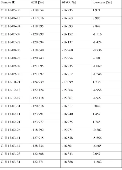
... 75 Table 6. δ2H, δ18O, and lc-excess values for all Con 1 groundwater and stream
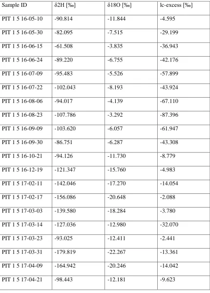
samples. C1E = main branch of Con 1 stream, C1S = groundwater spring near Con 1. ... 76 Table 7. δ2H, δ18O, and lc-excess values for all soil water samples. Pit 1 = hillslope
site, Pit 2 = riparian site. ... 79 Table 8. δ2H, δ18O, and lc-excess values for all plant samples. CC = hillslope
xi
LIST OF FIGURES
Figure 1. Dry Creek Experimental Watershed. From DCEW [2017]. ... 112 Figure 2. Instrumentation at Con 1 study site. Image taken from Geisler [2016]. Our
hillslope pit was located next to Con 1 Sap Flow and the riparian pit was located next to Con 1 East Gauge. ... 113 Figure 3. VWC data subset with diurnal signal. These signals were present in the
data from the 5 and 20 cm sensors, but not those deeper in the soil profile. ... 114 Figure 4. VWC and soil temperature subset. VWC diurnal fluctuations are in-phase
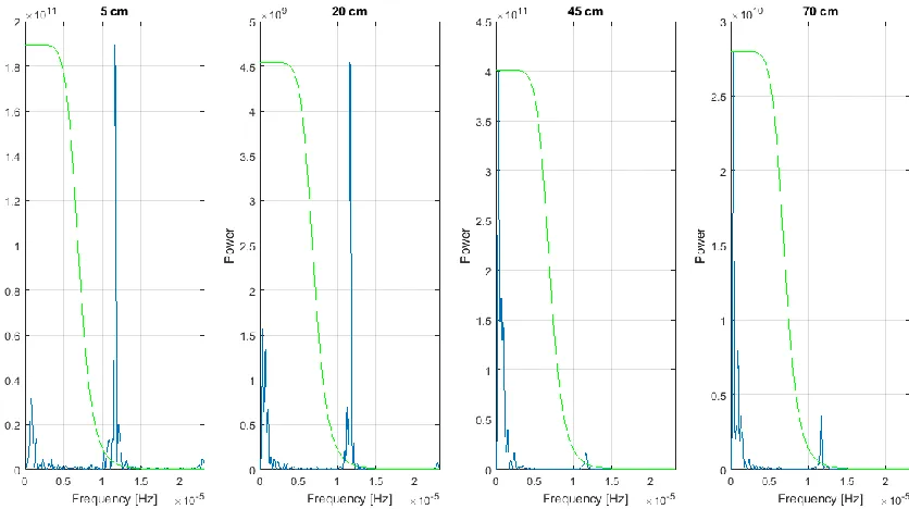
with and controlled by fluctuations in soil temperature. ... 115 Figure 5. Periodogram of VWC subset. Strong power spikes in 5 and 20 cm at 1.157
x 10-5 Hz correspond to a 24-hour period, confirming that the signal in these data is diurnal. ... 116 Figure 6. Periodogram of matric potential subset with low-pass filter. All data left of
the filter cutoff were conserved. ... 117 Figure 7. Subset of 5 cm matric potential data with results of low-pass filter. ... 118 Figure 8. Subset of matric potential and soil temperature. The two data sources are
out of phase. ... 119 Figure 9. Precipitation at Treeline hydrometerological station from March 1st, 2016
to July 31st, 2017 and at C1E station from March 1st, 2016 to April 1st, 2017 (top panel). No data was recorded after 4-1-2017 at C1E due to power issues. After this date, hydrometeorological data from the Treeline station were used as proxy. Time series of soil moisture and matric potential at the hillslope pit from May 2016 to July 2017 appear in the middle and bottom panels. The data gap in mid-June 2016 is due to power supply issues. The data gap in the 5 cm sensor and the drop in VWC in the 20 cm sensor in January 2017 is due to freezing soil conditions. Note that very small (0.001-0.002) residual diurnal fluctuations remain after
xii
presumably due to poor contact with the soil matrix due to dry conditions. ... 120 Figure 10. Time series of VWC at the riparian soil pit. Sensor malfunction,
particularly at 5 cm, resulted in missing data in late 2016 and early 2017. ... 121 Figure 11. Histograms of VWC sensor data. Bin count spikes at low VWC (< 0.05)
correspond to plant extraction limit. Bin count spikes at intermediate VWC (.10-.14) correspond to FC. Numeric results are reported in Table 1. ... 122 Figure 12. Characteristic moisture release curves generated by hillslope VWC and
matric potential data. ... 123 Figure 13. Characteristic curves generated from the Rosetta pedotransfer function and
in situ data. ... 124 Figure 14. δ2H and δ18O values for stream and groundwater sampled from 5-10-2016 to 7-6-17. Precipitation was sampled from 12-19-2016 to 6-13-17. ... 125 Figure 15. Lc-excess values for hillslope soil water in summer 2016 (top row),
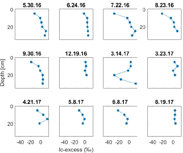
fall/winter 2016/2017 (middle row), and summer 2017 (bottom row). Note that some sampling dates are omitted from this figure to highlight general trends. ... 126 Figure 16. δ2H and δ18O values for hillslope and riparian soil water. ... 127
Figure 17. Lc-excess values for riparian soil water in summer 2016 (top row), fall/winter 2016/2017 (middle row), and spring 2017 (bottom row). Enriched lc-excess values are mostly restricted to the 5 cm layer. An enriched signal emerges at 20 and 25 cm on March 14th, 2017. This is likely due to extraction or sampling error. ... 128 Figure 18. δ2H and δ18O for hillslope soil water on May 10 and August 23, 2016. . 129
Figure 19. δ2H and δ18O for hillslope soil water at 70 cm or below during summer
2016. These data tightly cluster and do not move off the MWL over the growing season, suggesting minimal influence from more enriched layers higher in the soil column. These data overlap well with the groundwater data in Figure 14. ... 130 Figure 20. δ2H and δ18O for hillslope soil water on March 31st, 2017. ... 131 Figure 21. δ2H and δ18O for riparian soil water at 20 cm or below at selected dates
xiii
significantly about the plot over the growing season and overlap with stream and groundwater, suggesting minimal influence from more
enriched layers higher in the soil column. Upward movement of the water table to ~ 20 cm could also control isotopic composition in at these depths. ... 132 Figure 22. δ2H and δ18O for all plant species from May 2016 to July 2017……….133 Figure 23. Top panel: δ2H and δ18O for hillslope Douglas Fir and sagebrush from
May 10th through October 21st, 2016. Chokecherry was not sampled during this period. Middle panel: Hillslope Douglas Fir and sagebrush from December 19th, 2016, February 11th, and April 9th, 2017. Douglas Fir
and sagebrush moved progressively off the LMWL with each subsequent sampling date. Chokecherry was sampled on April 9th. Bottom Panel: Hillslope Douglas Fir, sagebrush and chokecherry from April 21st to July 6th, 2017. No directional trend existed in the data for any of the three species. The chokecherry data points in the upper right corner are from April 21st, possibly a vestige of winter enrichment before transpiration
began. ... 134 Figure 24. Top Panel: δ2H and δ18O for riparian Douglas Fir and water birch from
May 10th to September 30th, 2016. Middle Panel: Riparian Douglas Fir and water birch from December 19, 2016 to May 8th, 2017. Both species’
lowest lc-excess values occurred during this period. Bottom Panel:
Riparian Douglas Fir and water birch from May 24th to July 6th, 2017. . 135 Figure 25. Matric potential versus lc-excess at each sensor depth. Strong relationships
exist at 5 and 20 cm and virtually no relationship exists at the two lower depths. ... 136 Figure 26. Temporal evolution of matric potential versus lc-excess at 5 cm at the
hillslope pit. The most enriched soil water samples from summer 2016 are associated with the lowest matric potential values. The points along the x-axis suggest that elevated lc-excess (> -10 ‰) is not necessarily associated with lower matric potential, as some samples are associated with matric potential at or near estimated field capacity. ... 137 Figure 27. Temporal evolution of matric potential versus lc-excess at 20 cm at the
hillslope pit. Similar to the 5 cm layer, matric potential and isotopic enrichment coevolve throughout the study. At this depth, significantly enriched water (lc-excess > -10 ‰) is frequently immobile (< -10 kPa). ... 138 Figure 28. Temporal evolution of matric potential versus lc-excess at 45 cm at the
xiv
matric potential sensor at this depth malfunctioned around early
September 2016 until mid-December, presumably due to dry conditions. Three isotope sampling dates occurred in this period and all samples had lc-excess values < -5 ‰. These observations suggest that these samples would plot in the low lc-excess/high matric potential portion of the above plot. This would strengthen the conclusion that low matric potentials at this depth are not associated with enriched isotopic composition. ... 139 Figure 29. Temporal evolution of matric potential versus lc-excess at 70 cm at the
hillslope pit. The matric potential sensor at this depth malfunctioned around early October 2016 until February 2017, presumably due to dry conditions, as corroborated by the VWC data from this period. Three isotope sampling dates occurred in this period and all samples had lc-excess values < -10 ‰. These observations suggest that these samples would plot in the low lc-excess/high matric potential portion of the above plot. This would strengthen the conclusion that low matric potentials at this depth are not associated with enriched isotopic composition and that immobile water is not necessarily isotopically enriched. Most isotopic compositions cluster between lc-excess values of 5 and -10 ‰. Similar to the 45 cm water from the same period, early summer 2017 lc-excess values approach or slightly exceed significant enrichment (>-10 ‰) but are mostly associated with matric potentials near field capacity (~ -10 kPa). ... 140 Figure 30. VWC versus lc-excess at each sensor depth. As with Figure 36, strong
relationships exist at 5 and 20 cm and virtually no relationship exists at the two lower depths. Samples from 100 cm were not included due to small sample size. ... 141 Figure 31. Temporal evolution of VWC versus lc-excess at 5 cm at the hillslope pit.
The horizontal line represents field capacity as estimated by the frequency of occurrence method. The vertical line represents the threshold for significant isotopic enrichment as defined by the 95% CI for the LMWL. Labeled quadrants represent the following soil waters: I- enriched/mobile, II- unenriched/mobile, III- unenriched/immobile, IV- enriched/immobile. ... 142 Figure 32. Temporal evolution of VWC versus lc-excess at 20 cm at the hillslope pit. Almost all enriched water plots in Quadrant IV, while no soil water plots in Quadrant I. ... 143 Figure 33. Temporal evolution of VWC versus lc-excess at 45 cm at the hillslope pit.
... 144 Figure 34. Temporal evolution of VWC versus lc-excess at 70 cm at the hillslope pit.
xv
Figure 35. Time series of VWC at the hillslope pit from May 27th to July 24th, 2017. Dry down curve slope is similar in the 5, 20 and 45 cm sensors through mid-May. Two subsequent infiltration and dry down events show that curves are much steeper at 5 and 20 cm than for 45 cm. ... 146 Figure 36. Time series of soil temperature at the hillslope pit from May 12th, 2016 to
July 24th, 2017. ... 147 Figure 37. Soil water, VWC, and matric potential at the hillslope site from May 10th
to September 9th, 2016. Deep (> 70 cm) and shallow (< 15 cm) soil water isotopes from this time period are shown in Panel 1. ... 148 Figure 38. Time series of soil moisture at the hillslope pit from May 13th to May
22th, 2017. VWC increases progressively from 5 cm to 100 cm, with no sudden spikes at depth. This pattern was consistent for all infiltration events during the study period. ... 149 Figure 39. Soil water isotopes profiles at the hillslope site before and after July 10th,
2016 storm. ... 150 Figure 40. δ2H and δ18O for hillslope soil water on September 30th and October 21st,
2016. Shallow soil water isotopes move closer to the LMWL in response to fall rain. Deeper soil water becomes more enriched, but stays on the LMWL. ... 1511 Figure 41. Sap flux data from Con 1 site. Taken from Geisler [2016]. ... 152 Figure 42. δ2H and δ18O for hillslope soil water and hillslope sagebrush from July 9th
xvi
LIST OF ABBREVIATIONS AND SYMBOLS
C1E Confluence 1 East stream gaging location on Dry Creek C1S Confluence 1 groundwater spring
CI Confidence interval
Con 1 Primary field site in Dry Creek Experimental Watershed DCEW Dry Creek Experimental Watershed
ET Evapotranspiration
GMWL Global Meteoric Water Line LMWL Local Meteoric Water Line
VSMOW Vienna Standard Mean Ocean Water VWC Volumetric water content
INTRODUCTION
Stable isotopes of water have aided hydrologic investigations at a variety of scales. Naturally occurring isotopes have been used in tandem or independently to explore a variety of vadose zone processes including groundwater recharge [review by Koeniger et al., 2016], infiltration and mixing [Gat and Tzur, 1967; Gazis and Feng, 2004; Stumpp and Masloszewski, 2010; Zhao et al.,2013], plant water uptake [Brunel et al., 1991; Dawson, 1996; Gaines et al., 2016; Koeniger et al., 2010], and evaporation [Allison et al., 1983; Barnes and Allison, 1988]. Some of these processes alter soil water chemistry. For instance, evaporation enriches soil water in 2H and 18O, two commonly used isotopic tracers.
In addition to this evaporative enrichment, soil water mobility appears to decrease in drying soils. Mobility is most commonly defined by the volumetric water content and matric potential thresholds of field capacity that differentiate mobile from immobile water. Recent studies suggest that isotopically enriched soil water exists primarily as immobile water and this assumption has influenced interpretations of plant water isotopes. However, the strength of the relationship between VWC, matric potential and soil water isotopes remains poorly constrained. In this study, we investigate the
relationship between soil water mobility and soil water isotopic composition. A breadth of hydrological, biological, and geological processes occurs in
occur in these layers are referred to collectively as the plant-soil-atmosphere continuum. Thus, the vadose zone plays a critical role in partitioning precipitation into evaporation from soils, transpiration from plants and groundwater recharge. The processes by which precipitation is routed into these fluxes have important implications for solute transport [Nimmo, 2005], streamflow and groundwater dynamics, and plant productivity [Good et al., 2015]. Consequently, watershed model performance is partially dependent upon accurate representation of water infiltration and redistribution in the vadose zone.
Infiltration is most often discussed in the context of two conceptual frameworks, translatory flow and the mobile/immobile model. Hewlett and Hibbert[1967] asserted that water previously existing in a profile is displaced by infiltrating precipitation, a process also referred to as translatory or piston flow. However, there is considerable evidence that the translatory flow model does not fully explain all infiltration processes.
separation between mobile and immobile waters, estimating that only 38 % of surface runoff is derived from plant-accessible reservoirs.
Better understanding of soil water mobility is critical for constraining plant water uptake dynamics that can dominate water movement out of a watershed. Researchers explored plant uptake at least as far back as the early 18th century, with Hales’ [1727] studies of plant physiology. Jasechko et al., [2013] reported that plants account for 80 – 90% of total global evapotranspiration. If plants extract immobile soil waters that maintain different isotopic compositions from mobile water, such a finding would complicate hydrologic models that represent soil water as a single reservoir.
Recent studies suggest that plants and streams may indeed return different water pools to the hydrosphere. This idea was first referred to as the ‘two water worlds
hypothesis’ by McDonnell [2014] then renamed the ‘ecohydrological
compartmentalization hypothesis’ by Evaristo et al. [2015]. McCutcheon et al. [2017] referred to the two hypotheses collectively as the ‘ecohydrological separation
Evaluation of the ecohydrologic separation hypothesis is commonly determined through analysis of stable isotope composition of water samples, most frequently both 2H
and 18O ratios. In the context of the ecohydrologic separation studies mentioned previously, seasonal δ2H and δ18O variations in precipitation plot linearly to produce a
local meteoric water line [LMWL, Rozanski et al., 1992]. Stream and ground water plot on or very close to the LMWL, with seasonal variation along the line. Soil water that has experienced evaporation plots along a soil evaporation line with a lesser slope than the LMWL. Ecohydrologic separation is considered present when vegetation plots right of the LMWL and close to the soil evaporation line, rather than on the LMWL as would be expected if plants drew upon the same water pool that eventually contributes to
streamflow.
Despite growing evidence for the existence of ecohydrologic separation, several issues remain unresolved. Many field campaigns suffered from low temporal frequency of isotope sampling, particularly some of the earliest work on the subject [Brooks et al., 2010; Geris et al., 2015; Goldsmith et al.,2011]. In their review, Sprenger et al., [2016] noted that most field campaigns only sampled a few times per season and at a limited number of soil depths. Sprenger et al. [2017] demonstrated the utility of increased temporal and spatial sampling frequency in the Scottish Highlands to capture relatively weak evaporation signals in soil water.
[Oerter and Bowen, 2017] and even fewer use data from tensiometers or matric potential sensors [Song et al., 2009; Sprenger et al., 2016]to corroborate this assumption.
McCutcheon et al.[2017] demonstrated that some ecohydrologic separation research presupposes that soil water fates (plant uptake vs. drainage) can be used to identify soil water mobility, though these relationships remain poorly studied. The authors show that waters of the same mobility can differ in isotopic composition and that waters of similar isotopic composition can have differing mobility. Hence, the relationship between mobility and isotopic composition remains unclear, despite the prevailing interpretation of isotopic data.
There is a considerable need to evaluate ecohydrologic separation in semi-arid ecosystems. Despite the apparent ubiquity of ecohydrologic separation globally, 20% of the locations in Evaristo et al.[2015] showed no evidence of ecohydrologic separation. Likewise, Geris et al. [2015] reported limited evidence for ecohydrologic separation in a rainy, low energy environment in the Scottish boreal forest. Semi-arid and arid
which is also the location of our field site. However, no direct connection between
mobility and isotope composition was observed by the authors. McCutcheon et al. [2017] utilized VWC data present at several index sites in the watershed, but not at specific sampling sites.
The goal of this study is to define the relationship between soil water isotopic composition and soil water mobility. To improve temporal sampling frequency, we sampled soil, plant and stream water isotopes at least every 2-3 weeks during the dry-down period (April – July/August) of the 2016 and 2017 growing seasons and outside of these periods every 30-60 days. We installed VWC and matric potential sensors to
identify soil water retention characteristics of our sample site and to make more informed observations of soil water mobility on isotope sampling dates. Last, we gathered detailed soil texture information in consideration of recent studies that investigate the interplay between soil texture and soil water isotopic composition [Newberry et al., 2017b; Orlowski et al., 2016; Oshun et al., 2016].
Specific objectives of this study are to:
1) Assess seasonal evolution of soil water isotopic composition in a hillslope and riparian profile.
2) Determine the relationship between soil water mobility and isotopic composition.
SCIENTIFIC BACKGROUND
General Soil Water Dynamics
Soil moisture is a critical control on processes in the plant-soil-atmosphere interface, influencing the fluxes of evapotranspiration and groundwater recharge. Soil moisture is frequently expressed as a unitless value representing the volume of water per unit volume soil (m3/m3, VWC). Closely related to VWC is water potential, which is a
measure of potential energy at a given point in the subsurface. Water potential governs the ability of water to move from one area to another. Matric potential is the most important component of water potential in unsaturated soils and is frequently used to establish endpoints for water drainage and plant uptake to determine soil parameters. In unsaturated soils, soil water is held under tension or negative water potential.
Two VWC thresholds influence water fluxes in the vadose zone. The VWC at which drainage due to gravity ceases is termed field capacity [Veihmeyer and
Hendrickson, 1931]. Plant wilting point was defined as the VWC at which wilting occurs in plants by Briggs and Shantz [1912]. The accuracy of these terms has been questioned as far back as Miller and McMurdie[1953] and their utility is still being assessed
Precise determinations of field capacity are problematic since it is difficult to determine precisely when drainage due to gravity ends. Water potential values from -33 to -5 kPa have been suggested in the literature as the field capacity threshold, as reported by Chandler et al. [2017]. Most germane to this study, Romano and Santini[2002] established -10 kPa as the water potential corresponding to field capacity in coarse-grained soils. This value was supported by results from Chandler et al. [2017]. Constraining wilting point is difficult due to variation across plant species and soil texture. Wilting point is also complicated by the fact that incremental changes in VWC can result in relatively large changes in matric potential at the dry end of the
characteristic curves. Most studies use -1500 kPa to define wilting point, [Arslan et al., 2014; Monanty et al., 2015] but there is variation about this number. Seyfried et al. [2009] used plant extraction limit in place of wilting point, since transpiration in some species stops between -3000 and -5000 kPa with no apparent wilting [Chandler et al., 2017; Seyfried et al., 2009]. We use plant extraction limit here for this reason.
extraction limit. In addition, characteristic curves can provide information about soil water mobility by constraining field capacity and plant extraction limit thresholds. Defining Mobile and Immobile Soil Water
Varying definitions of mobile and immobile water exist in past studies and make inter-study comparisons difficult. The mobile-immobile model as originally proposed by Van Genutchen and Wieranga [1976] defines immobile water as that which does not actively drain and remains bound to the soil matrix. Landon et al. [1999] defined mobile water in temporal terms as ‘water entering the soil during the most recent precipitation or irrigation event’ and immobile as ‘water present in soil prior to most recent precipitation or irrigation event.’ Similarly, Gazis and Feng[2004] assumed that the immobile water portion is that which is not displaced after an infiltration event. These definitions may be physically accurate, but do not consider any VWC or tension thresholds to improve replicability. Zhao et al. [2013] employed a similar definition as Landon et al. [1999], but also proposed ‘a more specific definition of mobile pre-event water as the water
extractable with a suction lysimeter,’ though this definition is problematic for reasons discussed below. McCutcheon [2015] defined the mobile-immobile threshold as water above or below field capacity which is the definition employed here.
Sampling Mobile and Immobile Water
portion but did not employ any specific VWC thresholds for field capacity. Suction lysimeter extraction ranges frequently vary. Many suction lysimeters cannot sample water held below ~ -60 kPa, below field capacity but well above plant extraction limit. If the commonly accepted mobile-immobile threshold of -33 to -5 kPa is assumed, then studies using lysimeters set below this value extract water from both the mobile and immobile portion, assuming mobile water exists at the time of sampling. Berry et al. [2017] address this inconsistency by noting that variations in the lower limit of lysimeter extraction can lead to erroneous interpretations of ecohydrologic separation.
Sampling immobile soil water is often more problematic than sampling of mobile water. Because suction lysimeters cannot sample water held much below -60 kPa, many studies rely on destructive sampling of bulk soil water. An auger or other device is used to manually extract a plug of soil from a given depth from which water is then extracted through one of several laboratory methods discussed later. In situ assessments of field capacity and plant extraction limit thresholds are rarely used to help determine the relative mobility of a bulk soil sample. Gierke et al., [2016] used bulk samples to make inferences about immobile water but no VWC or water potential thresholds were
sampled waters. However, the basic tenets of the ecohydrologic separation hypothesis assert that isotopic signature can be used to determine infer mobility. If this is the case, then accurate observation of mobility would be unnecessary.
Water Isotope Analysis
Stable isotope distribution in the subsurface is controlled in part by stable isotope composition of precipitation. An empirical linear relationship exists between δ2H and δ18O composition in meteoric water.Rozanski et al., [1992] established a model for the
relationship of these stable water isotopes globally, termed the Global Meteoric Water Line (GMWL) and defined as:
δ2H = 8.2 * δ18O + 11.27
Local meteorological conditions affect the relationship established by the GMWL. Therefore, a Local Meteoric Water Line (LMWL) is more commonly used in watershed isotopic analyses and often differs slightly from the GMWL in slope and intercept.
Evaporation of water can take place under equilibrium (relative humidity ≈ 100%) or non-equilibrium conditions (relative humidity < 100%). Lighter isotopologues
an increased accumulation of 18O relative to 2H in the residual water [Craig et al.,1963]. Water experiencing non-equilibrium fractionation plots to the right of the GMWL. Soil Water Isotope Dynamics
Stable isotopes of water are increasingly used to study hydrological processes at a variety of scales but controls on isotopic composition of soil pore water remain poorly understood [McDonnell, 2014; Sprenger et al., 2016;]. These isotopes are considered conservative tracers given that the tracer is the water molecule itself. Zimmerman et al. [1967b] was among first to use stable isotopes of soil water to explore soil moisture dynamics. In their review, Sprenger et al. [2016] demonstrated that isotopic analyses are useful at the catchment, hillslope and profile scale. Uniform volumetric and isotopic input at the plot scale is assumed in most cases, though spatio-temporal variation almost
certainly exists [Sprenger et al., 2016]. Generally, spatial heterogeneity in soil water isotopes is much greater in the vertical direction than horizontal [Brooks et al., 2010; Zhao et al., 2013].
lysimeter-extracted water plotted on the LMWL and bulk water did not, suggesting that evaporation from the mobile water compartment occurs under equilibrium conditions’ and that non-equilibrium evaporation occurs after ‘water has been adsorbed/absorbed in soil particles.’ This description is analogous to first-stage and second-stage evaporation, as described by Or et al. [2013] and Dingman[2015].
Infiltration Mechanisms and Soil Water Isotopes
Controls on infiltration in a soil profile include soil texture [Stumpp and Maloszewski, 2010], the existence or absence of preferential flowpaths [Stumpp and Maloszewski, 2010; Beven and Germann, 2013], vegetation [Liu et al., 2015], antecedent moisture conditions [Gazis and Feng, 2004; Dahlke et al., 2012], and duration and
magnitude of precipitation event [Gazis and Feng, 2004]. Infiltration is most often described in terms of two distinct end-members: piston or diffuse flow, in which water systematically moves downward in a relatively uniform wetting front [Hewlett and Hibbert, 1967] and preferential flow, in which infiltrating water bypasses upper soil layers via larger soil pores [Beven and Germann, 1982]. Myriad isotope-based studies corroborate the existence of preferential flowpaths [Mueller et al., 2014; Stumpp and Maloszewski, 2010; Gazis and Feng, 2004; Liu et al., 2015; Mathieu and Baric, 1996]. Still others found evidence for both piston and preferential flow in the same soil profile [Ma et al., 2017; review by Beven and Germann, 2013; Song et al.,2009; Mathieu and Baric, 1996]. Zhao et al.[2013] noted both preferential flow and diffuse flow in soils in southwestern China, with piston flow dominating during high antecedent moisture conditions.
diffuse flow dominated below the root zone in grass and heather. Zhao et al.[2013] observed the opposite effect as piston flow dominated in the grass-dominated upper soil layers and preferential flow through macropores drained soil in layers lower than 20 cm.
Isotope Sampling of Vegetation
Stable isotope studies in vegetation commonly assume that no fractionation of soil water takes place during uptake based on studies including Allison et al., [1984],
Zimmerman et al.[1967a] and Zhang et al. [2010]. Studies show that sapwood,
heartwood [White et al., 1985] and plant cellulose isotopic composition matched that of source water [Rodan and Ehleringer, 1999]. Likewise, evaporation from suberized stems has long been considered negligible [Geris et al., 2017 via Ehleringer and Dawson, 1992]. Brunel et al. [1991] found no significant isotopic differences in twig samples versus water from the main stem. This effect is likely due to the relative volume of xylem versus bark and phloem.
More recent studies have shown evidence of fractionation within plant tissues [Zhao et al., 2016] or selective uptake of lighter isotopes in plant water. Ellsworth and Williams [2007] found variations of up to 0.2 ‰ in δ18O between bark and xylem samples and δ2H variations up to 6 ‰ between the two tissues in Prosopis velutina, a
woody xerophyte.The authors propose that symplastic uptake pathways contribute to fractionation specifically in xerophytes and halophytes. Results from Vargas et al. [2017] were interpreted to imply preferential uptake of lighter isotopes by avocado plants, leaving soil water with an enriched composition.
Plant water isotope interpretations between studies are complicated by
studies [Beyer et al., 2016; Herve-Fernandez et al., 2016; Goldsmith et al., 2011; McCutcheon et al.,2015; White et al., 1985]. Twig cuttings are commonly used when coring is impossible due to plant size or species growth habit. Twig cuttings are extracted with the bark removed [Brunel et al., 1991; Oerter and Bowen, 2017; Vargas et al., 2017], intact [McCutcheon et al.,2015] or not specified as removed or intact [Geris et al., 2017; Herve-Fernandez et al., 2016]. Still other studies sample transpired water [Beyer et al., 2016] or leaves [Piayda et al., 2017] and back-calculate xylem water composition. Isotope extraction methods
METHODS
Approach
To track isotopic evolution, we sampled soil, plant and stream water isotopes from May 2016 to July 2017. We installed VWC and matric potential sensors at two locations to identify soil water retention characteristics of our sample site and to make more informed observations of soil water mobility on isotope sampling dates. Last, we gathered detailed soil texture information that was used to model soil characteristic curves for comparison to field data.
Study Site Description
Dry Creek Experimental Watershed (DCEW, Figure 1) is a 27 km2 research catchment located approximately 16 km north of Boise, ID. Elevation ranges from 950 m at Dry Creek’s outlet near Bogus Basin Road to 2130 m at Bogus Basin ski area. The main branch of Dry Creek flows generally southwest and is subject to seasonal loss of flow at lower elevations. Shingle Creek is the only perennial tributary, though multiple ephemeral streams and springs exist in winter through late spring.
DCEW has a semi-arid climate with moderately cold to cold winters and hot, dry summers [DCEW, 2017]. Average precipitation in DCEW is highly dependent on elevation, with around 400 mm falling at lower elevations and 900 mm at upper
precipitation occurs between November and April. Most winter precipitation falls as snow in upper elevations and a rain/snow mixture or rain in lower elevations of DCEW.
The Atlanta Lobe of the Idaho Batholith underlies DCEW. This Cretaceous-aged unit is approximately 75 to 85 million years old [Johnson et al., 1988]. The predominate rock type in DCEW is medium to coarse-grained fractured biotite granodiorite. Soils in DCEW form from in situ weathering of the underlying bedrock. Smith[2010] reported soil types in DCEW hillslopes as loamy sands and sands, both with high gravel contents. DCEW[2017] states that DCEW soils range from loam to sandy loam.
Vegetation communities in DCEW are dependent on aspect, elevation and proximity to the riparian zone. A sagebrush steppe community of cheatgrass (Bromus tectorum) and big sagebrush (Artemisia tridentate) dominate most aspects of lower elevations. Ponderosa pine (Pinus ponderosa) and Douglas fir (Pseudotsuga menziesii) predominate on most aspects in upper elevations with scattered populations of deciduous species such as aspen (Populus tremuloides) and chokecherry (Prunus virginiana). Middle elevations serve as an ecotone between the lowland sagebrush steppe community and conifer-dominated uplands. Riparian areas host considerably more biomass and diversity than hillslopes [McCutcheon, 2015]. Predominate riparian species include water birch (Betula occidentalis), yellow willow (Salix lutea) and Pacific willow (Salix lucida). Refer to McCutcheon [2015] for more detailed information regarding vegetation
distribution in DCEW.
Several watershed-scale studies have quantified the contribution of discharge and ET to the water balance of DCEW. Stratton et al. [2009] applied the Soil Water
and 2007, respectively. Aishlin and McNamara[2011] used a chloride mass balance to calculate ET withdrawals as high as 70 % for the 2005-2009 water years. For water years 2002-2011, Parham [2015] used hypsometrically distributed precipitation data to estimate ET at 48% of total precipitation. Geisler [2016] noted that much of DCEW is water-limited during the growing season, and that potential ET is generally higher than actual ET.
General Description of Con 1 Study Site
For this study, we chose the Con 1 site in DCEW (Figure 2) due to its previous use in BSU ecohydrological studies and its unique vegetation communities. Con 1 is located at 1335 m at the transition between sagebrush steppe and mixed
conifer-deciduous forest, which allowed us to sample plant species from both communities. We accessed Con 1 via a pullout off Bogus Basin Road near the DCEW Treeline site. From this point, Con 1 is located down a ~1.5 km trail with 250 m of elevation loss.
Stream discharge has been recorded at Con 1 since 2004 [DCEW, 2017].Geisler [2016] installed sap flux sensors in multiple plant species on both the hillslope and in the riparian zone. A meteorological station with a tipping bucket precipitation gage was also installed by Geisler[2016] and we used these data to identify precipitation timing and magnitude from 5-10-16 to 2017. A power failure at this station occurred on 3-31-17. After this date, we used hydrometeorological data from the DCEW Treeline site where necessary.
saturated zone. The second profile was located in the riparian zone ~2 m from the north bank of C1E (riparian site). Slope was < 5° at the riparian pit.
Instrumentation
To assess VWC changes within the soil profile, we dug a 100 cm pit at the hillslope site. Digging was impractical below this point due to impenetrable rock. We inserted Campbell Scientific CS655 soil water content reflectometers into the pit wall at 5, 20, 45, 70 and 100 cm to assess changes in VWC and soil temperature over time. The CS655 sensors were connected to a Campbell Scientific CS6 data logger. At the riparian site, we dug a 25 cm soil pit. The saturated zone began at 20 cm on the installation date. CS655 VWC sensors were placed at 5 and 25 cm in the pit wall. At both sites, we took pains to backfill soil in the original layers maintained before excavation.
The CS655 sensors measured VWC every 60 seconds and the data logger averaged these readings every 15 minutes from May 10, 2016 to September 30th, 2017. The CS6 data logger compiled the averaged readings to produce time series of VWC at each sensor depth. After September 30th, 2016, we programmed sensors to take readings every five minutes and the data logger to average these readings hourly. We decreased the sampling rate due to decreased battery life with the onset of colder weather. Our observations up to this point showed that hourly measurements were sufficient to identify sub-daily trends in soil moisture, which was more than adequate for our research goals. Analytical precision of CS655 sensors is 0.05 % and VWC accuracy is ± 3 % of reading [Campbell Scientific, 2017]. The resulting soil moisture time series were further
We acknowledge that VWC sensors placed at 5 cm likely underestimate soil moisture because the sensing volume extends slightly above the ground surface at this depth [Campbell Scientific, 2017]. We chose this depth to constrain infiltration timing and detect low-volume precipitation inputs rather than the most accurate volumetric measurements.
We placed Decagon MPS-6 calibrated matric potential sensors at depths of 5, 20, 45, and 70 cm in the hillslope soil pit. These depths corresponded with our four
uppermost VWC sensors. We made small excavations in the pit face and placed the MPS-6 units into these openings to ensure maximum connectivity to the soil matrix. The MPS-6 units measure the moisture content of a ceramic disc with a known moisture-matric potential relationship. These moisture content sensors use changes in dielectric permittivity to determine VWC, similar to the functionality of the CS-655 VWC sensors. The range of the MPS-6 sensors is -9 kPa to -100,000 kPa. Measurement accuracy for the MPS-6 sensors is ± 10 % of the reading between -9 kPa and -100 kPa, and Decagon Devices reports good sensor-to-sensor agreement and accuracy down to -1500 kPa. Below -1500 kPa, validation with other measurement sources is difficult, but Decagon [2017] suggests that accuracy in this range is around 25%. For calibration standards and general information on the MPS-6 units, refer to Decagon[2017].
Soil Sampling for Grain Size Distribution
profile. At the riparian site, one bulk soil sample was taken at each sensor depth. The soil core sampler was not used at the riparian site due to excessive root density throughout the profile past the water table. All soil samples were sealed in Ziploc bags and transported back to the BSU Soils Lab.
Bags were left open for one month, then placed in a 105° C oven for two days to ensure complete drying. Samples were weighed then broken up using a mortar and pestle to discourage clumping and to homogenize any root mass. Root mass was negligible in all hillslope samples except those collected at 5 cm.
We tested all soil samples for total organic carbon using the loss on ignition method. Loss on ignition is commonly used in soil studies as an inexpensive and easy way to measure organic carbon in soil samples [Ball, 1964; Goldin, 1997]. We removed a 5 g subsample from each bag and placed it in a muffle furnace at 375° C for 16 hours as described by [Robertson, 2011]. We calculated mass lost over this time to determine soil organic carbon content.
We sieved the entire soil sample (minus 5 g for loss on ignition) using the
The results from grain size distribution analysis were used to model water release curves using the artificial neural network Rosetta, as described by Schaap et al. [1998, 2001]. Calibration of the Rosetta network was performed using samples from temperate climate zones of the northern hemisphere. Rosetta solves for van Genuchten parameters as below [van Genuchten, 1980]:
θ(h) = θr + (θs – θr) / (1 + │αh│n)1-1/n
where θ(h) defines the characteristic curve which relates θ [cm3/cm3] as a function of the
soil water pressure head h [cm], also referred to as capillary pressure or matric potential [Guber and Pechepsky, 2010]. θr and θs [cm3/cm3] are residual and saturated water
contents, while α (1/cm) and n are curve shape parameters. We compared the modeled curves to the field curves generated by the in situ VWC and MP sensors.
Liquid Water Sampling
Pennsylvania. Our precipitation samples reflect net isotopic composition over a single storm cycle and do not address any intra-storm variations.
We sampled stream water at the C1E gaging station immediately adjacent to the riparian site. Twenty mL scintillation bottles were filled completely then capped for transport from the field. A small spring (C1S) enters Dry Creek near Con 1. We sampled water from this spring as above to use as a proxy for groundwater isotopic composition. C1S dried completely from late summer to late fall 2016 and we gathered no samples during this time.
Soil and Plant Sampling for Isotopic Composition
To investigate isotopic evolution within our soil profiles, we gathered soil samples beginning in May 2016. Since sampling in the sensor-soil interface was impossible, we took pains to sample within ~4 meters of the VWC and matric potential installations. We used an open-bit auger (5 cm x 20 cm) and sampled every 5 cm until we encountered impenetrable rock, usually between 70 and 100 cm at the hillslope site. We usually encountered standing water and/or impenetrable roots at 20 or 25 cm at the riparian site. One sample was taken at each depth to manage extraction and analysis time and costs, though we acknowledge some spatial heterogeneity likely exists even at this small scale as observed by Sprenger et al. [2017]. Soil samples from each depth were immediately transferred from the auger to a 19x150 mm test tube to discourage isotopic fractionation. We capped and sealed samples for transport to BSU.
sagebrush, SB2 was sampled after this date. SB1 data were not used in this study. From February to July 2017 at the hillslope site, we sampled a chokecherry specimen to investigate a deciduous species. At the riparian site, cuttings were taken from a Douglas fir and water birch. Plants were sampled roughly every two weeks from May to October 2016, once a month from November 2016 to April 2017, and every two weeks from April 2017 to July 2017.
For all species, we selected mature, suberized branches to minimize any possible isotopic fractionation suspected in new growth [Ehleringer and Dawson, 1992]. Douglas fir cuttings were taken at roughly breast height. Water birch samples were taken from breast height to ~ 6 feet from tree base due to preponderance of sample-size branches in this range. Samples were cut as close to the main stem as possible, then quickly cut into ~ 1 cm pieces with the bark intact. We stored plant samples in 19x150 mm test tubes that were capped and sealed for transport to BSU.
In the field, we stored plant, soil and liquid water samples in a small cooler that contained dry ice or frozen water bottles to prevent evaporation. Upon return from the field, we immediately placed samples in a -20⁰ C freezer until extraction. Precipitation, stream water and groundwater samples were stored at 4⁰ C to prevent explosion of glass containers. Total time between sample collection and transfer to cold storage was no more than five hours, which minimized any evaporative effects.
Water Extraction: Cryogenic Vacuum Distillation
The system consists of eight U-shaped stainless steel units which each accommodate two 19x150 mm test tubes. Two test tubes fit tightly in each end of the unit, one containing a plant or soil sample, the other empty. Each unit is connected to a stainless steel manifold which is attached to a pump. This apparatus achieves pressures as low as 15 millitor when not in active use.
We used tweezers to remove any plant material from the soil samples. A plug of glass wool was placed in the top of each soil sample test tube to prevent any soil from being drawn into the system during pumping. Glass wool is non-reactive during extraction [Newberry et al., 2017a]. We submerged test tubes containing plant and soil samples in liquid nitrogen for two minutes to immobilize our sample before pumping. The pump system created pressures of 20-30 millitor between the sample test tube and the empty tube. Swagelock valves were closed above each unit to maintain these
pressures. We placed the sample test tubes in small furnaces that maintained temperatures of 100⁰ C to evaporate water within the samples. We were careful to keep furnace
temperatures below 105° C to avoid possible liberation of water from soil mineral structure [Sacchi et al, 2000]. The empty test tube was submerged in liquid nitrogen for the duration of extraction. Water vapor was drawn into the empty test tube from the sample test tube where it froze to the empty test tube wall.
Plant samples were extracted for 60 minutes and soil samples for 45 minutes. These extraction times were chosen based on lab experiments by West et al. [2006], Orlowski et al.[2013] and Jia et al., [2012]. The original sample test tubes were examined after extraction was completed. We noticed a very small number (< 5)
this was due to loss of pressure inside these units and we discarded these samples. When extraction was completed, we removed the test tubes from liquid nitrogen and allowed them to reach room temperature until all ice had melted in the extracted water. We transferred the extracted water into 12x35 mmvials and stored them at -20⁰C until analysis.
Plant and Soil Water Isotopic Analysis
All water samples were analyzed for isotopic composition on a ThermoFisher High Temperature Conversion Elemental Analyzer connected to a Delta V+ Isotope Ratio Mass Spectrometer. These units were housed at the BSU Stable Isotope Laboratory. Standard deviation of measurements of a reference gas for δ18O and δ2H was 0.08‰and
0.27 ‰, respectively. We used four water standards with known δ18O and δ2H values during sample runs to determine instrument accuracy and repeatability of results. These standards were chosen to represent the breadth of isotopic compositions expected in our samples. Standard deviation from the four standards was 0.51, 0.41, 0.54 and 0.38 ‰ for δ18O and 1.94, 2.28, 1.86, and 1.46 ‰ for δ2H. Isotope values are reported in parts per
mil (‰) as calculated below:
δ2H or δ18O = [R
sample / RVSMOW – 1] * 1000
where Rsample = 2H/1H or 18O/16O and RVSMOW is the isotope ratio of the standard, Vienna
Isotope Data Analysis
For data visualization in dual isotope plots, we used the LMWL derived for the Treeline location by McCutcheon[2015], based on data collected and weighting factors determined by Tappa [2013] and McCutcheon [2015]:
δ2 H = 7.70 * δ18 O + 4.95
For isotopic composition comparisons, we use line-conditioned excess (lc-excess) as described by Landwehr and Coplen [2006] and defined as:
lc-excess = δ2 H - a * δ18 O - b
where a and b represent the slope and intercept of the LMWL. This means that lc-excess is the vertical distance from the LMWL of a sample as measured by δ2 H deviation.
Lc-excess of precipitation is 0 ‰ by definition, making it a preferable metric for assessing deviation from the MWL [Sprenger et al., 2017]. Ecohydrologic separation studies commonly employ a combination of dual-isotope plots and lc-excess, as waters can share similar lc-excess values but very different combinations of δ2H and δ18O.
VWC and matric potential temperature correction
on permittivity of the soil matrix. Campbell Scientific[2017] notes that CS655 sensors first measure permittivity then use the Topp equation to derive VWC. Since VWC sensors depend upon permittivity to measure VWC, soil temperature-induced changes in permittivity can be recorded incorrectly as changes in VWC. We hypothesized that our VWC data displayed a temperature-induced diurnal signal.
To confirm our visual assessment of VWC changes over 24-hour cycles, we isolated a rainless subset of the soil moisture data from August 17th to September 28th,
2016. This subset was selected due to minimal linear trends in VWC over this period. We generated a periodogramto analyze this data subset at all sensor depths. This analysis revealed a periodicity of 24.008 hours for the 5 and 20 cm sensors (Figure 5). The periodogram showed that daily soil temperature fluctuations at the 45, 70 and 100 cm depths were too small to influence the VWC data.
We temperature-corrected the raw VWC data as described by Cobos and Campbell [2007]. This method was intended to guide temperature correction of data obtained by Decagon ECH2O soil moisture sensors. Although we used CS655 sensors in
this study, their functionality is similar to the ECH2O sensors. Both sensor types derive
VWC data from measurements of permittivity, which is temperature dependent as
described above. Neither Decagon Devices nor Campbell Scientific noted either sensor to be sensitive to soil temperature changes. We feel confident that application of this
temperature correction method to the CS655 data discussed here is justified.
all data with a period lower than this cutoff value. Virtually no data were removed other than those with a 24-hour period as shown in Figure 6. This method eliminated the diurnal signal in the tension data (Figure 7). Inconsistencies between the original and filtered data occurred during periods of rapid wetting or drying. We considered the corrected data suitable for subsequent analysis because these periods did not coincide with isotope sampling. For more information on the use of Butterworth filters refer to Roberts and Roberts[1978].
There is speculation that diurnal fluctuations in VWC and matric potential are tied to plant water uptake during the day and hydraulic redistribution at night [Mares et al., 2016]. However, our data show an increase in VWC and matric potential during the daytime (Figures 4 and 8). This observation runs counter to the idea that plants are inducing a diurnal decrease in both VWC and matric potential due to daytime
transpiration. Therefore, we feel confident that removal of diurnal signals in both datasets is justified.
VWC Data Processing and Generation of Characteristic Curves
throughout the study period. The processed VWC data were plotted in a histogram to determine field capacity and plant extraction limitas described by Chandler et al. [2017].
RESULTS VWC Trends
General soil moisture trends (Figure 9) were consistent with previous
observations of seasonal precipitation in the Boise Foothills (DCEW, 2017). The 5 and 20 cm sensors showed sensitivity to large-scale precipitation events. The 45, 70, and 100 cm sensors showed steady dry-down in summer, followed by steady wet-up in winter before dry-down began again in early summer 2017. A steady dry-down of all VWC sensors marked the summer months. A single significant infiltration event (July 10th, 2016) occurred between mid-May and late-September. Occasional storms of light intensity and duration (< 2 mm per hour for 1-2 hours) occurred over this period (Figure 9). However, the July 10th infiltration event only affected the 5 and 20 cm VWC sensors. Progressive wet-up of the hillslope soil profile occurred beginning in late September with the 5 and 20 cm sensors. The wetting front did not reach the 70 and 100 cm sensors until mid-winter 2017. The hillslope location was snow-covered from at least December 19th,
2016 to March 11th, 2017. All snow cover after this point was intermittent.
Estimation of Field Capacity and Plant Extraction Limit
Estimated values for field capacity and plant extraction limit derived from the frequency analysis method in Chandler et al. [2017] are shown in Figure 11and Table 3.
Plant extraction limit is much more clearly defined in the frequency analysis than field capacity. Plant extraction limit values from frequency analysis show mostly good agreement with those derived from in situ characteristic curves. Plant extraction limit derived from the Rosetta model were systematically higher than those from frequency analysis. Plant extraction limit from frequency analysis corresponds to the lowest VWC values recorded over the study, with values ranging from 0.01 to 0.04.
We used -33 kPa for estimating field capacity from the in situ characteristic curves since the wettest VWC values clustered around -10 kPa, making it difficult to distinguish an appropriate value. Field capacity ranged from 0.10 – 0.14 for the five sensor depths and values show good agreement with those derived from the Rosetta model, but relatively poor agreement with the values from the characteristic curves. These values appear less constrained than plant extraction limit from frequency analysis, with multiple spikes for several sensors. As noted previously, a subset of the 5 and 20 cm VWC data was removed due to complications from below freezing soil temperatures. The timing of these complications was unfortunate as VWC was expected to stabilize during this period and would have helped constrain field capacity estimates. Despite this issue, these field capacity estimations provide adequate baselines for further analysis.
limit. The soil profile drained quickly back to or near field capacity during infiltration events (< 1 week), even during periods when there was likely little or no transpiration, such as early spring 2017.
Matric Potential Trends
Soil matric potential generally tracked changes in VWC (Figure 9). Matric potential at 45 and 70 cm showed a very steady dry-down from -10 kPa in May 2016 to less than -5000 kPa in September 2016. Dry conditions were assumed to exist through early winter but were not recorded due to sensor failure. A very rapid increase in matric potential in December (45 cm) and February (70 cm) occurred when the wetting front reached these sensors, as corroborated by the VWC data. Summer dry-down began again in May 2017. The 5 cm and 20 cm data were more variable than the deeper sensors and experienced repeated shallow infiltration events and evaporation cycles. During summer 2016 and 2017 dry-down, matric potential decreased at a slower rate for the 5 and 20 cm sensors versus those at 45 and 70 cm, and much higher values were recorded at deeper sensors in early fall (~ -5000 kPa vs. -2000 kPa). Fall rains increased matric potential for the 5 and 20 cm sensors to ~ -10 kPa, where it remained until the summer 2017 dry-down began in May.
Grain Size Analysis and Rosetta Results
sand with organic carbon from 1.5 – 2.9 %. The B-horizon was weakly formed where it existed at all. Virtually no clay (1% or less) was detected in the soil samples
corresponding to the locations of our sensors. Below 40-45 cm, coarse pebbles and small cobbles of the parent granitics were occasionally encountered. The 70 cm layer was mostly composed of saprolite and had organic carbon percentages at or below 1 % and contained 91-93% sand-sized particles.
Riparian soils were categorized as sands with low silt content (< 7%) and virtually no clay content (<1%). Organic carbon levels were several percentage points higher at the riparian site than at the hillslope site.
Characteristic curves generated from VWC and MP data show hysteresis in wetting and drying limbs at all depths (Figure 12). The data from 5 and 20 cm show multiple wetting and drying cycles and drying limbs do not always overlap one another. The 45 and 70-cm curves show only one wetting and one drying cycle, though these main wetting and drying limbs occupy different areas of the plot and do not overlap. Wetting curves of the two deepest sensors are characterized by large decreases in tension with very small (< 0.01) increases in VWC in winter 2017. The 5-cm curve is shifted left relative to the other sensors, likely due to underestimation of VWC as discussed previously in the Methods section.
period at these depths. The curves from the 45 and 70 cm depths showed much better agreement, though matric potential was consistently underestimated.
Isotopic Trends in Precipitation, Stream and Groundwater
Precipitation samples plot along the LMWL with no significant deviations as shown in Figure 14. The mean δ2H and δ18O values were -104.62 (σ = 32.44) and -14.06 (σ = 3.61), respectively. Winter samples plot lower on the MWL than do spring and early summer samples. However, they are not arranged linearly with time of precipitation. For example, the 4-9-17 rain/snow mix plots higher up the MWL than does the 6-19-17 rain event.
Like previous ecohydrologic separation studies [Bowling et al., 2016; Brooks et al.,2010; Oshun et al., 2016], stream and groundwater samples clustered tightly on the MWL and varied little seasonally (Figure 14). Mean δ2H and δ18O for stream water was
-121.53 (σ = 2.74) and -16.26 (σ = 0.48), respectively. Mean δ2H and δ18O for
groundwater was -122.54 (σ = 3.22) and -16.14 (σ = 0.54), respectively. Isotopic Trends in Soil Water
Mean δ2H and δ18O for all soil water was -121.90 (σ = 16.48) and -15.47 (σ = 2.93). Mean δ2H and δ18O for hillslope soil water was -122.55 (σ = 17.53) and -15.41 (σ = 3.07). Upper soil layers showed considerably more variation relative to lower layers through summer 2016 (Figure 15). This phenomenon was also observed by Song et al., [2009], McCutcheon et al., [2017], and Zhao et al., [2013]. Lc-excess became
-10, indicating minimal effects from evaporation or movement of high lc-excess water lower in the soil profile. Increased precipitation and VWC in fall 2016 coincided with lc-excess values near zero at all depths from October 2016 through March 2017 (Figure 15). 5 cm water from 3-14-17 is highly enriched, possibly due to the last melt input from an enriched snowpack.
Hillslope soil profiles from late spring 2017 (Figure 15) show more isotopic variability with decreasing depth as observed by Ma et al.[2017], Song et al., [2009] and Zhao et al.,[2013]. As shown in Figure 9, the months of March and April 2017 were the wettest period of the study. No soil layers have highly negative (< -20) lc-excess values until June 8th, and these are restricted to the 5 cm layer. Subsequent rain storms on June 11-12th dilute this signal in the 5 and 10 cm layers of the June 19th profile. Curiously, shallow layers (< 30 cm) occasionally show negative lcexcess values between 20 and -10 ‰.
Riparian soil water varied less than hillslope soil water in both δ2H and δ18O
(Figure 16). Mean δ2H and δ18O for riparian soil water was 124.25 (σ = 11.47) and -16.36 (σ = 1.87). Evaporative enrichment was restricted to the 5 cm layer but lc-excess values never exceeded -40 ‰ (Figure 17). The enriched signal at 5 cm was absent in the December 19th profile (Figure 17). A highly enriched signal at 20 and 25 cm (lc-excess > -20) emerged on March 14th, 2017 but was absent on March 23rd, at least down to 20 cm.
Riparian soil isotopes from late spring to early summer had lc-excess values generally less negative than -10 ‰ (Figure 17).
enriched on the MWL than lower layers (Figure 18). Shallow soil water from late summer 2016 shows a trend along an evaporation line (Figure 18) as observed in many studies including McCutcheon et al. [2017] and simulations by Sprenger et al. [2016]. Considering the findings of Benettin et al. [2018], we refer to an apparent soil
evaporation line, but make no inferences from it regarding source water. As the summer months progress, the deepest (> 70 cm) soil water generally occupies the same location on dual isotope plots, with minimal movement up and down the MWL and no movement off it (Figure 19). By 12-19-16, all soil water plots on the MWL, but without the linear structure observed on 5-10-2016. Soil water clusters at its lowest point on the MWL on February 17, 2016 and moves up the MWL from late winter through early spring. Spring 2017 was very wet, with alternating rain and quickly-melting snow storms. The resulting soil water plots change dramatically between sample dates over this period, particularly in the shallowest layers. Shallow soil water from a few sampling dates plot outside of the 95% CI for the MWL. For the March 31st and April 9th profiles (Figure 20), these
unexpected compositions may be the result of precipitation that falls on a MWL with a steeper slope in the winter months as observed by Tappa [2013].
Deep (> 20 cm) riparian soil water plots near stream and groundwater for the duration of the study period (Figure 21), except for the anomaly from March 14th, 2017 (Figure 17).
Isotopic Trends in Hillslope Plant Water
sagebrush was -125.05 (σ = 7.55), -14.33 (σ = 1.7) and -19.77 (σ = 10.36). McCutcheon et al. [2017] also noted the least negative lc-excess values in Douglas Fir versus
sagebrush and deciduous species in DCEW. Dual isotope plots of plant water reveal that hillslope Douglas Fir water plots within or just below the LMWL 95% CI from May 10th to October 21st, 2016 (Figure 23), similar to the trend observed by McCutcheon et al. [2017] and Gierke et al. [2016]. Sagebrush water plots inside the LMWL 95% CI through the June 15th sampling date but moves off beginning July 9th through October 21st.
Sagebrush water makes a distinct move back towards the LMWL on 12-19-17 and 2-11-17 but maintains an enriched composition.
The 2-11-17 and 4-9-17 hillslope Douglas Fir water plots off the LMWL with lc-excess values around -20 (Figure 23). Similarly, the 4-9-17 sagebrush water possesses higher lc-excess values (-33 and -35) than Douglas Fir, plotting well right of the LMWL. This date is also the first sampling date for chokecherry, which had lc-excess values below -30 as well. Mean δ2H, δ18O, and lc-excess for hillslope chokecherry was -131.81
(σ = 11.39), -15.64 (σ = 2.79) and -16.39 (σ = 11.25).
Isotopic Trends in Riparian Plant Water
Mean δ2H, δ18O, and lcexcess for riparian Douglas Fir was 128.27 (σ = 8.64),
-16.28 (σ = 1.54), and -7.92 (σ = 9.74), respectively. Mean δ2H and δ18O for riparian water
birch was -127.15 (σ = 9.31), -14.92 (σ = 2.21), and -17.22 (σ = 10.56), respectively. Dual isotope plots show that both species plot mostly right of the LMWL but within the 95% CI from 5-10-16 to 8-6-16. A weak evaporative signal emerged in water birch (lc-excess > -20 ‰) until September 30th when lc-excess averaged -27.4 (Figure 24). The
DISCUSSION
The Relationship Between Mobility and Isotopic Composition
To assess the relationship between isotopic composition and soil water mobility, we plotted lc-excess of soil water sampled at each sensor depth against matric potential (Figure 25). Strong positive relationships exist at 5 and 20 cm as matric potential
decreases with increasingly negative lc-excess. Examination of the seasonal evolution of isotopic content and matric potential at 5 and 20 cm reveals that the highest lc-excess and lowest matric potentials at these depths occurred in late summer 2016 (Figures 26 and 27). Early summer 2017 samples suggest the continuation of this trend.
No relationship exists between isotopic composition and matric potential at the 45 and 70 cm depths (Figures 28 and 29). Matric potentials at these depths were
systematically higher than shallower depths over the same period, but isotopic
enrichment was restricted to lc-excess values below -20 and mostly below -10 ‰. These results are similar to the observations by McCutcheon et al. [2017] of waters with similar isotopic composition held at varying tensions.