http://www.sciencepublishinggroup.com/j/ijics doi: 10.11648/j.ijics.20180304.11
ISSN: 2575-1700 (Print); ISSN: 2575-1719 (Online)
Quality Verification of Audio and Image Modulation by the
Simulation of PCM, DM and DPCM Systems
Gaby Abou Haidar, Roger Achkar, Hasan Dourgham
Department of Computer and Communications Engineering, American University of Science and Technology, Beirut, Lebanon
Email address:
To cite this article:
Gaby Abou Haidar, Roger Achkar, Hasan Dourgham. Quality Verification of Audio and Image Modulation by the Simulation of PCM, DM and DPCM Systems. International Journal of Information and Communication Sciences. Vol. 3, No. 4, 2018, pp. 110-120.
doi: 10.11648/j.ijics.20180304.11
Received: February 28, 2019; Accepted: April 4, 2019; Published: May 8, 2019
Abstract:
Modulation is a process through which a message has to pass in order to be effectively transmitted. However, there are some limitations to Pulse Code Modulation and Delta Modulation that can cause data redundancy, quantization error, slope overload distortion and granular noise which result in a bad communication process. Throughout the past few years, Pulse Code Modulation (PCM), Delta Modulation (DM) and Differential Pulse Code Modulation (DPCM), in digital communication systems, have proven to have unparalleled advantages over analog communication systems; this is in terms of error minimization and distances of transmission enhancements. Delta Modulation, a simplified version of Pulse Coded Modulation also pauses major problems in noise and quantization error. Consequently, and to combat the arising problems, communication engineers have developed newly adaptive compression and modulations techniques for better digital transmission. One of these innovative systems is the Differential Pulse Coded Modulation (DPCM) that can solve the aforementioned problems. Thus the focal point of this article is to explore the simulation of these systems using Simulink (The Math Works, Inc., USA). Eventually, the systems are tested on both image and audio inputs to prove the superiority of DPCM over DM and PCM systems in reducing noise and increasing the signal to quantization noise ratio, thus insuring a smooth and successful transfer of data.Keywords:
Pulse Coded Modulation, Differential Pulse Coded Modulation, Adaptive Prediction, Simulink1. Introduction
Digital communication is the transfer of data over a point-to-point or even point-to-multipoint communication channel (copper wires, optical fibers, and wireless communications media). Moreover, those systems usually use a digital sequence as an interface between the source and the channel input, as well as between the channel output and the final destination. Nowadays, digital communication systems are considered as standards to transmit data from a source to specific destination through a channel [1]. The importance of such communication systems relies on many qualifications and mainly on the simplification of such systems. For example, source coding/decoding can be done independently of the channel. Similarly, channel coding/decoding can be done independently from the source [2].
Several modulation techniques do exist in digital communication systems in order to make data feasible for
remarks and possible extensions of the presented work.
2. Background Information
For a long time, PCM was the only digital communication system when transmitting data through a channel. However, the quantization error in such a system results in the generation of noise and distortion in the transmitted data. Consequently, DPCM was invented to solve the problems of the PCM system. So, what are PCM and DPCM? Why is there a generation of noise in PCM? What is the importance of DPCM systems?
This article covers three types of modulation techniques in digital communication: Pulse code modulation, Delta Modulation and Differential Pulse-Code Modulation. Somehow, the process of modulation in all of the three techniques is the same in theory. The transmission of the signal consists mainly of two parts: modulation and demodulation [5].
The modulation phase consists mainly of three steps: Sampling, Quantization and Encoding. Sampling is the process of measuring the amplitude of a continuous-time signal at discrete instants, and converting these continuous signals into a discrete signal. For example, conversion of a sound wave to a sequence of samples.
Figure 1. Analog and Sampled Signal.
Figure 2. Quantized Signal.
Quantization is dividing the range of possible values of the analog samples into different levels, and assigning the center value of each level to any sample in quantization interval. Quantization approximates the analog sample values with the nearest quantization values. Almost all the quantized samples will differ from the original samples by a small amount. That amount is called as quantization error. The quantization interval or quantization step size is known as Q [5].
Finally, the encoder encodes the quantized samples. Each quantized sample is encoded into an 8-bit code word. In DPCM only the difference between a sample and the previous value is encoded. The difference is much smaller than the total sample value, so less number of bits is needed for getting the same accuracy as in ordinary PCM. In this case, the required bit rate will also reduce.
The demodulation phase is the reverse of the modulation phase. At the receiver end, a demodulator decodes the binary signal back into pulses with the same quantum levels as those in the modulator. By further processes, the original analog waveform can be restored.
2.1. Pulse Coded Modulation (PCM)
Pulse Coded Modulation (PCM) is a method used to digitally represent sampled analog signals; in PCM a signal is represented by a sequence of coded pulses. A PCM stream is an analog signal represented in digits. The magnitude of the analog signal is sampled regularly at uniform intervals, with each sample being quantized to the nearest value within a range of digital steps [6].
PCM has been used in digital telephone systems and is also the standard form for digital audio in computers and compact disks. However, PCM is not typically used for video in consumer applications such as DVD and DVR because it requires two high bit rates [6].
The performance of a PCM system is influenced by two major sources of noise: the quantization noise which is introduced in the transmitter and is carried all the way to the receiver output, and the channel noise which is introduced anywhere between the transmitter and the receiver. This noise disappears when the message signal is switched off, making this signal dependent [3, 7].
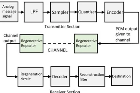
The basic operations performed by the PCM transmitter are: sampling in which the signal is changed into a discrete time signal; quantizing in which the discrete values are approximated and changed into levels, and encoding in which the obtained levels are changed to bits. As for the PCM receiver, it consists of the decoder that changes the obtained bits to levels again, and the reconstruction filter that reconstructs the original signal [8]. The block diagram of PCM system is shown in “Figure 3”.
More into equation wise, the formula derived for the quantization can be stated as:
[ ] q[ ] [ ]
q n =x n −x n (1)
Where q[n] is the quantization error, x[n] the original signal, and xq[n] of the quantized signal. The maximum quantization error is simply max(|q|), the absolute maximum of this error function which can be written as:
1 max( ) min( )
2N
x x
Q= −+ (2)
2.2. Delta Modulation (DM)
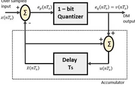
Delta Modulation is a simplified version of Pulse Coded Modulation. The output of a delta modulator is a bit stream of samples, at a relatively high rate. The value of each bit is determined according to whether the input message sample amplitude has increased or decreased relative to the previous sample. Delta modulator operates in the following manner: it samples periodically the input message, makes a comparison of the current sample with that preceding it, and then outputs a single bit which indicates the sign of difference between the two samples. This, in principle, would require a sample-and-hold type circuit. Figure 4 illustrates the basic system in block diagram form.
Figure 4. DM System Block Diagram.
The system is in the form of a feedback loop. This means that its operation is not necessarily obvious, and its analysis is non-trivial. However, it can still be built, and it can still operate in the manner a delta modulator should. The system is a continuous time system to discrete time converter. In fact, it is a form of analog to digital converter. It is the starting point from which more sophisticated delta modulators can be
developed.
In delta modulation, there is a restriction on the amplitude of the input signal. The reason behind that is the large derivative of the transmitted signal (Abrupt changes). In this case, a modulated signal cannot follow the input signal and Slope Overload occurs. This can be mathematically represented as follows. Consider having the following input signal:
( ) cos ( )
m t =A t ωt (3)
Modulated Signal (Derivative of Input Signal) which is transmitted by the Modulator:
.
max
( )
m t =ωA (4)
Whereas the condition to avoid Slope Overload is:
.
max
( ) s
m t =ωA<σf (5)
So Maximum Amplitude of Input signal can be:
max s
f
A σ
ω
= (6)
Where fs is Sampling Frequency and ω is the Frequency of the input Signal and σ is Step Size in Quantization. So, Amax is the Maximum Amplitude that DM can transmit without causing the Slope Overload, and the Power of Transmitted Signal depends on the Maximum Amplitude [9].
2.3. Differential Pulse Coded Modulation (DPCM)
Differential Pulse Coded Modulation (DPCM) is a signal encoder that uses the baseline of Pulse Coded Modulation (PCM), but adds some functionality based on the prediction of the future values of the signal. A difference relative to the output of a local model of the decoder process is taken instead of taking a difference relative to the previous input sample. In this latter option, the difference can be quantized, securing a good way to incorporate a controlled loss in the encoding. Thus, the DPCM system reduces the error generated by the quantization process (known as the “quantization error”) at the transmitter of the PCM system. The DPCM transmitter is similar to the PCM transmitter, but it has a prediction filter for predicting the future values of the signal in order to eliminate the quantization error [10].
Concerning the Signal to Noise Ratio (SNR), it is much improved in the case of DPCM over the PCM. This allows much better noise filtering with less bandwidth; for example, if we have two signals m(t) and d(t) with M and D being their peak amplitudes respectively, and if the same quantization level L is used to sample both signals, the quantization step ∆υ in DPCM is reduced by a factor of / . The corresponding quantization noise power is ∆υ^2 /2
factor / ^2; since the SNR is inversely proportional to noise, it increases by the same factor [11]. In Practice, the SNR improvement may be as high as 25 dB leading to short-term voiced speech spectra. Alternatively, for the same SNR, the bit rate for DPCM could be lower than PCM by 3 to 4 bits per sample. This reduces the bandwidth. DPCM system block diagram is shown in “Figure 5”.
Figure 5. DPCM System Block Diagram.
Working in equation wise form, then the prediction error is to be written as:
ˆ [ ] [ ] [ ]
e n =m n −m n (7)
Now the reconstruction equation can be written as: ˆq[ ] q[ ] ˆ[ ]
m n =e n +m n (8)
And finally, the reconstruction error equation which is computed the same way as the quantization error as be written as:
ˆ [ ]q [ ] q[ ] [ ]
m n −m n =e n +e n =q (9)
In practice, DPCM is usually used with lossy compression techniques, like coarser quantization of differences can be used, which leads to shorter code words. This is used in JPEG and in adaptive DPCM (ADPCM), a common audio compression method. ADPCM can be watched as a superset of DPCM.
3. Audio Simulation Using Simulink
The audio compression theory studied in this paper covers three different systems: PCM, DM and DPCM. The simulation and compression of audio in Simulink are presented in this section.
3.1. Simulink Implementation of Audio Pulse Coded Modulation
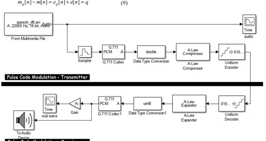
The implementation of pulse coded modulation (PCM) for audio in Simulink, as shown in “Figure 6”, requires the following: an audio that can be inserted using “from multimedia block” that provides the signal to be tested; a sampler to sample the continuous signal at a rate greater than or equal to the Nyquist rate [12]; G.711 codec PCM block which is an International Telecommunication Union for audio companding; an A-law(or µ-law) compressor along with a uniform encoder to encode the obtained levels to a bit data stream; and a decoder with an A-law (or µ-law) expander followed by a G.711 codec again to reconstruct the original signal. The audio can be heard using “to audio” block from Simulink by setting it first after the original signal, and finally after the gain. In addition, vector scopes are added in order to visualize the graphs under each part where the signal is passing through.
3.2. Simulink Implementation of Audio Delta Modulation
The Simulink implementation of delta modulation (DM), as shown in “Figure 7”, consists of the following blocks: an audio that is considered as the input signal to be tested, a
sampler, a quantizer for the quantization process, an integrator along with a uniform encoder for the encoding process, and a uniform decoder with an integrator and a low pass filter to reconstruct the original signal.
Figure 7. DM System for Audio Modulation.
3.3. Simulink Implementation of Audio Differential Pulse Coded Modulation
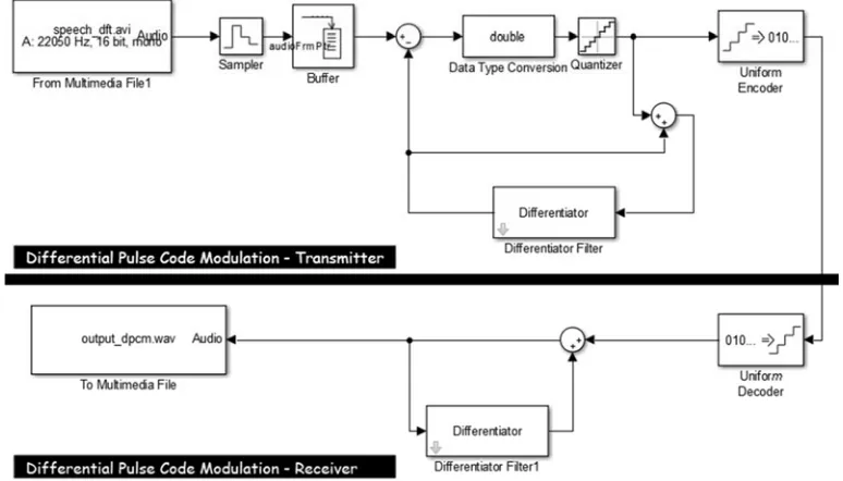
The Simulink implementation of differential pulse coded modulation (DPCM), as shown in “Figure 8”, consists of the following blocks: an audio that is considered as the input
signal to be tested, a sampler, a quantizer for the quantization process, a differentiator filter that acts as a prediction filter along with a uniform encoder for the encoding process, and a uniform decoder with a differentiator filter again to reconstruct the original signal.
Figure 8. DPCM System for Audio Modulation.
4. Simulation Results - Audio
After the implementation of PCM, DM and DPCM systems on the audio input, the results are visualized on the vector spectrum for the audio. As shown in “Figure9”, the
moving the audio into the output after the process of quantization took place, the audio heard is noisy. This shows a clear presence of disturbance that might be solved by the prediction and feedback filters presented in the DPCM system. But, this is still a theory until it is tested. So, does the DPCM give better results when it comes to audio simulation?
Figure 9. PCM, DM & DPCM Audio Input Spectrum.
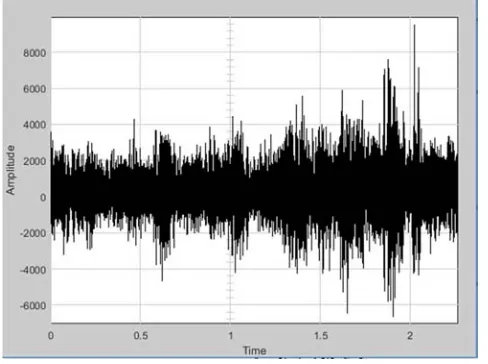
Comparing this spectrum to the PCM audio spectrum at the output, as shown in “Figure 10”, it is clear that the peak is reached at least four times per frame, and the amplitude fluctuates between 7000 and -6000. Besides, the peaks are reached at wrong times as the spectrum amplitude reaches 6500 almost all the time. These peaks and the amplitude fluctuations ensure the presence of noise and the quantization error in PCM system that affect the received audio negatively compared to the input image, which is only 3000 at peak in the first second.
Figure 10. PCM Audio Output Spectrum.
Moreover, comparing the output of the DM audio spectrum, shown in “Figure 11”, to both the input and the PCM audio output spectrum, it is obvious that the peak (8000) is reached many times as the audio elongates into the 700 frames; thus, the noise is not reduced from the PCM, and the
output contains less noise than the PCM but so much noise compared to the input audio.
Figure 11. DM Audio Output Spectrum.
Furthermore, comparing the output of the DPCM audio spectrum, shown in “Figure 12”, to the input of the PCM and the DM audio output spectrum, it is obvious that the peak (8000) is only reached twice in the last frames and in the rest. The amplitude fluctuates between 3000 and -2000; therefore, the noise is absolutely reduced from the PCM and DM and the output is approximately the same as the input. The output spectrum shows several peaks as well, which ensures that the noise still exists in the DPCM system while compressing the audio. However, the noise is reduced compared to the other two systems PCM and DM.
Figure 12. DPCM Audio Output Spectrum.
5. Image Simulation Using Simulink
Image simulation using Simulink consists of several steps using both Matlab workspace and Simulink.
Step 1: Loading image to be processed into Matlab workspace using RGB = imread('x.png').
Step 2: Transforming the image from an RGB to grayscale using I = rgb2gray(RGB)
Step 3: The images were then binarised, so they could exist in a solely black and white (monochrome) format. This was achieved by performing a “nearest color” thresholding method [13], which ensured that each grey level of the original image could be matched to the closer of the two binary colors. Binarisation was also performed so that reduction of similar training pairs could be more easily executed in further steps.
This step reduces statistical redundancy of the image and exploits perceptual irrelevancy. It reduces transmission time and storage requirement with increase in transmission rate
[14].
Step 4: Loading the binerised image from Matlab workspace into Simulink models to be processed.
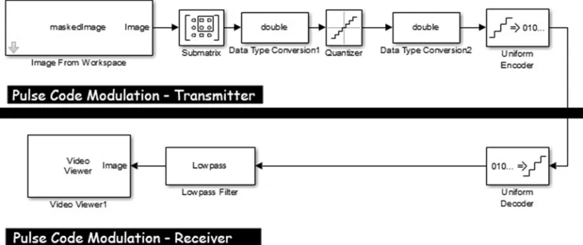
5.1. Simulink Implementation of Image Pulse Coded Modulation
The Simulink implementation of image pulse coded modulation, as shown in “Figure 13”, consists of the following blocks: an image that can be inserted using “Image from workspace” block, and that can provide the input to be tested, a submatrix block that transforms the image into a discrete format (acts here as a sampler), a quantizer block to quantize and encoder to encode the signal (the parameters of this block has to be designed perfectly in order to fit the image and its quantization), and a decoder with a low-pass filter to reconstruct the original signal. The image can be viewed using a video viewer block.
Figure 13. PCM System for Image Modulation.
5.2. Simulink Implementation of Image Delta Modulation
The Simulink implementation of image digital pulse coded modulation, shown in “Figure 14”, consists of the following blocks: an input which is the image, a submatrix block to
sample the image into very small pixels (acts here as a sampler), a quantizer and encoder along with an integrator, and a decoder again with an integrator to reconstruct the original signal.
5.3. Simulink Implementation of Image Digital Pulse Coded Modulation
The Simulink implementation of image digital pulse coded modulation, shown in “Figure 15”, consists of the following blocks: an input which is the image, a submatrix block to
sample the image into a very small pixels, a quantizer and encoder along with a prediction filter that is here a Kalman Filter (order 3), and a decoder with a Kalman Filter (order 3) to reconstruct the original signal [15, 16]. The image can be viewed using a video viewer block.
Figure 15. DPCM System of Image Modulation.
Image processing in Matlab and Simulink will take some time considering the long algebraic loop that the Matlab has to solve. The processing time will vary according to the number of pixels in the image and the image dimensions. If the image is used in gray scale without being binerised, Matlab will take a lot of time to process the image due to the differences in the number of pixels [17].
6. Simulation Results - Image
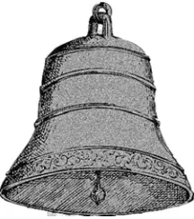
The system is tested in both: binerised and non-binerised images. When it comes to the processing of image in PCM, DM and DPCM systems in a non-binerised image, the results are as follows: comparing the image in “Figure 16” – bell.jpg (70x70), which is an input image for the three systems.
Figure 16. PCM, DM & DPCM Input Image.
to that in “Figure 17”, which is a PCM system output, it is
obvious that there exists a quantity of noise in the modulation due to the quantization error.
Figure 17. PCM Output Image.
However, comparing “Figure 18”, which is the output of the DM system, to the other two figures, the conclusion drawn is that the image is pixelated but it is clearer in colors and view from the PCM.
However, comparing “Figure 19”, which is the output of the DPCM system, to the other figures, the conclusion drawn is that the image is little bit pixelated but it is much more neat than that of the PCM and DM and also approximately the same as the input image.
Figure 19. DPCM Output Image.
For a binerised image, two images were processed in the three systems: the arrow.png image “Figure 20”and the calendar.png image “Figure 21”. The arrow.png image is a 27x27 image and 900 bytes’ size.
Figure 20. Arrow.png Image.
The calendar.png image is a 40x40 image of 2353 bytes.
Figure 21. Calendar.png Image.
The PSNR block in Simulink computes the peak signal-to-noise ratio, in decibels, between two images. This ratio is often used as a quality measurement between the original and a compressed image.
The Mean Square Error (MSE) and the Peak Signal to Noise Ratio (PSNR) are the two error metrics used to compare image compression quality. The MSE represents the cumulative squared error between the compressed and the original image, whereas PSNR represents a measure of the peak error. The lower the value of MSE, the lower the error [18].
To compute the PSNR, the block first calculates the mean-squared error using the following equation:
∑ , , ,
∗ (10)
In the previous equation, M and N are the number of rows and columns in the input images, respectively. Then the block computes the PSNR using the following equation:
10 !"#$%&'() (11)
In the previous equation, R is the maximum fluctuation in the input image data type. For example, if the input image has a double-precision floating-point data type, then R is 1. If it has an 8-bit unsigned integer data type, R is 255, etc. [19, 20].
The MSE is calculated in the Matlab workspace using the following equation:
err=immse(ReconstructedImage, IinputImage); (12) Where the ReconstructedImage is saved the workspace after building and running each of the three systems and InputImage is loaded to the workspace from the simulation folder.
Starting with the Arrow.png image, the image was processed and compressed in the three systems. The PCM system output is presented in the following Figure
Figure 22. Compressed Arrow.png in PCM System.
The PSNR is found to be 20.32 dB with an output image compressed to 233 bytes and thus 74% compression ratio. The MSE is computed and found to be 12732.6984 in the PCM system.
The DM system reconstructed image or compressed arrow image is presented in “Figure 23”. The image is better constructed with less error than the image compressed using PCM System.
Figure 23. Compressed Arrow.png in DM System.
The calculated PSNR and MSE of the DM system for the arrow.png image compression are 5.554 dB and 251.7421 respectively. The compression rate increases to 80.5% (176 bytes). These values change for the better when compressing the image in a DPCM system. The PSNR calculated is 2.085 and the MSE is 250.12. The compression rate is found to be the best between the three systems which is 81%. The compressed arrow image using DPCM is presented in “Figure 24”.
Figure 24. Compressed Arrow.png in DPCM System.
The testing of the three systems on a larger scale image (Calendar.png) verified the results obtained when testing in the Arrow.png image.
Table 1. Calnedar.png Image Compression Calculate MSE, PSNR and Compression Ration in PCM, DM and DPCM.
Type of Modulation MSE PSNR (in dB) Compression Ratio
PCM 21755.297 22.22 524 bytes 78%
DM 364.4239 6.897 197 bytes 91%
DPCM 300.12 3.371 194 bytes92%
The reconstructed images of the Calendar.png image after being processed in the PCM, DM and DPCM systems are presented in the table below. The best compression results with respect to the image quality are absolutely those obtained from the DPCM system. The least quality with respect to the compression ratio are those obtained after the PCM system.
Table 2. Compressed Calendar Image in PCM, DM and DPCM Systems.
Type of Modulation Compressed Image
PCM
DM
DPCM
7. Conclusions and Future Work
The work in this article shows the importance of certain modulation techniques as Differential Pulse Code Modulation in some environments and in solving errors resulting from commonly used modulation techniques as the Pulse Coded Modulation. Optimizing the predictor and the quantizer components are the basics when designing a DPCM system. Because the inclusion of the quantizer in the prediction loop results in a complex dependency between the prediction error and the quantization error, a joint optimization should ideally be performed. The power in the DPCM relies on its prediction filter that is capable of predicting the next state of the input based on the interaction with a pre-specified number of filters. The prediction helps in minimizing the quantization error and in removing the granular noise which is caused by PCM systems. Thus, a typical example of a signal good for DPCM is a line in a continuous-tone (photographic) image which mostly contains smooth tone transitions. Another example would be an audio signal with a low-biased frequency spectrum.
The significance of this work is that it shows three well- known modulation techniques that are simulated using Simulink with different types of inputs (pictures, voice and testing signals) rather than using the Simulink for testing normal signal generated from a block, or using the Matlab code for ordinary simulation done through many other researches. The Simulink blocks are built in a customized way trying to minimize the error distortion and optimize the quality of the output. This is achieved especially when using DPCM with an adaptive feedback predictor and a well-designed quantizer. The outputs show that DPCM is a powerful modulation technique if designed in a proper way.
As for future recommendations, the design of the predictor has to be well-defined and tuned for optimal results to be achieved. In addition, some new techniques, such as neural networks, can be used to enhance the adaptivity of DPCM and ADPCM.
Acknowledgements
Special thanks goes to all colleagues and professors at AUST to their various beneficial contributions for the project entitled “Quality Verification of Audio and Image Modulation by the Simulation of PCM, DM and DPCM Systems”. This work is in continuous support by the American University of Science and Technology.
References
[1] Simon Haykin. “Communication Systems”, New York: John Wiley and Son, Inc., 2000.
[2] Robert Galloger. “Introduction to Digital Communications”, Internet: http://ocw.mit.edu/courses/electrical-engineering-and-computer science /6-450-principles-of-digital-communications-i-fall-2006/lecture-notes / book_1.pdf, [Jun. 25, 2015].
[3] C. Mansour, R. Achkar, G. Abou Haidar “Simulation of DPCM and ADM Systems”, IEEE 14th International Conference on Modelling and Simulation, UKSim 2012 Cambridge, United Kingdom March 28-30, pp. 416-421. [4] G. Abou Haidar, R. Achkar and H. Dourgham, “A
Comparative Simulation Study of the Real Effect of PCM & DPCM Systems on Audio and Image Modulation” IEEE International Multidisciplinary Conference on Engineering Technology (IMCET 2016), Beirut, Lebanon, 2-4 November 2016, pp 144-149.
[5] Widrow, J. Glover, J. M. McCool, J. Kaunitz, C. S. Williams, H.Hearn, J. R. Zeidler, E.Dong, and R. Goodlin,“Adaptive noise cancelling: Principles and applications ”, Proc. IEEE, vol. 63, pp.1692-1716, Dec. 1975.
[6] William N. Waggener (1999). “Pulse Code Modulation Systems
[7] Design”, 1st ed., Boston, MA: Artech House.
[8] B.M Oliver, J.R Pirece, and C.E Shannon. “The Philosophy of PCM”. Proceeding of the IRE 36.
[9] N. S. Jayant and A. E. Rosenberg. "The Preference of Slope Overload to Granularity in the Delta Modulation of Speech". The Bell System Technical Journal, Volume 50, no. 10, December 1971.
[11] Institute of Radio Engineers, vol. 37, no. 1 pp 10-21.
[12] Dony, R. D., and Haykin, S., (1995), Neural Network Approaches to Image Compression, Proceedings of the IEEE, Vol. 23, No. 2, pp 289-303.
[13] Egger O, Fleury P, Ebrahimi T, Kunt M (1999) High-Performance Compression of Visual Information-A Tutorial Review-Part I: Still Pictures. In: Proceedings of the IEEE, vol. 87, no 6, June 1999.
[14] M. J. Weinberger, G. Seroussi and G. Sapiro, The LOCO-I Lossless Image Compression Algorithm: Principles and Sta- ndardization into JPEG-LS, IEEE Transaction on Image Processing, Vol. 9, No. 8, 2000, pp. 1309-1324.
[15] G. W. Cottrell and P. Munro, “Principal components analysis of images via back propagation,” in SPIE Vol. 1001 Visual Communications and Image Processing ’88, 1988, pp. 1070– 1077.
[16] Nelson, M., (1991), The Data Compression Book, M & T Publishing Inc.
[17] T. Acharya and A. K. Ray, Image Processing: Principles and Applications. Hoboken, NJ: John Wiley & Sons, 2005. [18] Chafic Saide, R´egis Lengelle, Paul Honeine, C´edric Richard,
and Roger Achkar. Nonlinear adaptive filtering using kernel-based algorithms with dictionary adaptation. International Journal of Adaptive Control and Signal Processing, 29(11):1391–1410, 2015.
[19] S Jayaraman, S Esakkirajan, T Veerakumar, “Digital Image Processing”, Tata Mc Graw Hill Educaation Private Limited, 2009.
[20] Noll P (1997) MPEG digital audio coding. In: IEEE Signal Processing Magazine vol 14, no 5, pp. 59-81, Sept 1997. [21] Scott Umbaugh, “Computer Vision and Image Processing”,
Prentice Hal Intl., Inc., 1988.
[22] R. C. Gonzalez, R. E. Woods and S. L. Eddins, Digital Image Processing Using MATLAB, (Pearson Edition, Dorling Kindersley, London, 2003).
Biography
Gaby Abou Haidar Coordinator of the Faculty of Engineering at AUST- Zahle. Mr. Abou Haidar got his M.S. degree in Computer and Communications Engineering from the American University of Science and Technology AUST- Lebanon in 2008. He completed the Microsoft Certified System Engineer MCSE program in 2005 and was officially employed as an I.T Manager and a CCE- lab instructor at AUST-Zahle in 2008. His responsibility is to teach major Engineering Labs. Moreover, he teaches the Computer Networking course, Virtual Instrumentation Systems, Digital Communications, and Embedded Systems. In 2009 he was CISCO certified as a (CCNA and CCNAS) instructor. Currently, Mr. Abou Haidar is finishing his Ph.D. degree at the University of Bordeaux –France in the field of Fractional Control Systems.
Roger Achkar Dean of the Faculty of Engineering at the American University of Science and Technology and an Associate Professor in Electrical Engineering. Dr. Achkar received a Ph.D. degree in Energetic System and Information from the University of Technology of Compiegne, France, in 2008. A Master degree in Research (DEA) from the Lebanese University, Faculty of Engineering, in 2004, and a B.E degree in Electrical Engineering from the Lebanese University, Faculty of Engineering, Branch II, Roumieh, Lebanon, in 2002. Dr. Achkar has been a member of the Order of Engineers and Architects in Lebanon since 2005, and Treasurer of the IEEE Lebanon Section. His Research interests are in Electrical, Communications and Mechanical Engineering Education. He developed and applied, on an active magnetic bearing (AMB), an artificial neural network able to control non-linear systems. Currently, he is leading several research projects in the area of Artificial Intelligence, Machine Learning, IOT, Communications, Vision and Control.