Variable Neighborhood Search for solving Bandwidth
Coloring Problem
Dragan Mati´c1, Jozef Kratica2, and Vladimir Filipovi´c3
1 Faculty of Mathematics and Natural Sciences, Mladena Stojanovi´ca 2 78000 Banjaluka, Bosnia and Herzegovina
Mathematical Institute of the Serbian Academy of Sciences and Arts, 11000 Belgrade, Serbia
Faculty of Mathematics, Studentski trg 16 11000 Belgrade, Serbia
Abstract. This paper presents a variable neighborhood search (VNS) algorithm for solving bandwidth coloring problem (BCP) and bandwidth multicoloring problem (BMCP). BCP and BMCP are generalizations of the well known vertex coloring problem and they are of a great interest from both theoretical and practical points of view. Presented VNS combines a shaking procedure which perturbs the colors for an increasing number of vertices and a specific variable neighborhood descent (VND) procedure, based on the specially designed arrangement of the vertices which are the subject of re-coloring. By this approach, local search is split in a series of dis-joint procedures, enabling better choice of the vertices which are addressed to re-color. The experiments performed on the geometric graphs from the literature show that proposed method is highly competitive with the state-of-the-art algorithms and improves 2 out of 33 previous best known solutions for BMCP.
Keywords: Bandwidth Coloring, Bandwidth MultiColoring, Frequency Assign-ment, Variable Neighborhood Search, Variable Neighborhood Descent
1.
Introduction
Vertex coloring problem (VCP) and its generalizations belong to a well known and widely researched class of graph coloring problems. Various generalizations and variants of VCP have been researched over the years and there are thousands of scientific papers proposing various methods for solving VCP and its generalizations.
In VCP, one needs to color the vertices of the graph in such a way that adjacent ver-tices must be colored with different colors and the aim is to minimize the number of used colors. During the years, as one of the most studied NP-hard combinatorial opti-mization problems, VCP has undergone many generalizations. This paper deals with two generalizations of VCP: bandwidth coloring problem (BCP) and bandwidth multicoloring problem (BMCP).
BCP is a straightforward generalization of VCP, where for each two adjacent vertices
uandvthe distance,d(u, v)is imposed and the difference between two colors assigned
assumed to be the set of consecutive integers{1,2, ..., k}and the task of BCP is to color
the vertices by colors from the set of available colors, where the numberkis as small as
possible.
Formally, for a graphG = (V, E)with positive integer distance function d(u, v),
(u, v)∈E, the objective of BCP is to find the coloringc:V → {1,2, ..., k}such that for each pair of adjacent verticesuandv,|c(u)−c(v)| ≥d(u, v)and the total numberkof used colors is minimized. Obviously, if the distance between any pair of adjacent vertices is equal to 1, BCP is brought down to VCP.
BMCP generalizes BCP by including the multicoloring of the vertices. For each vertex
vin the input graph a positive integer weightw(v)is given, holding the information how many colors must be assigned to that vertex. Additionally, distance between the vertex to
itself is also given, holding the condition inherited from BCP. Formally, letG= (V, E)
be a graph with positive integer weights on verticesw(v), v ∈ V and positive integer
distance functiond(u, v), (u, v)∈E. In the caseu=v, the valued(u, u)associated to
the loop edge(u, u), represents the minimum distance between different colors assigned
to the same vertexu. A feasible coloring in BMCP is defined as follows: to each vertex
u∈V, one needs to assign a setc(u)of total ofw(u)distinct colors, such that for each edge(u, v) ∈ E holds(∀p ∈ c(u))(∀q ∈ c(v))(|p−q| ≥ d(u, v)), i.e. the difference
between any colors of verticesuandv must be not less than the distance associated to
the edge(u, v). In the case of loop edges (u = v), the condition (∀p, q ∈ c(u), p 6=
q)(|p−q| ≥ d(u, u))must be satisfied. BMCP is reduced to BCP if for each vertexu
holdsw(u) = 1.
BMCP can be converted into BCP, by splitting each vertexvinto a clique of
cardinal-ityw(v). Each edge in the clique is assigned the distanced(u, u), corresponding to the distance of the loop edge of the vertexuin the original graph. By this approach, each
in-stance of BMCP, withnvertices, is transformed to the instance of BCP, havingPn
i=1w(i)
vertices. This fact leads to the approach of constructing the algorithm for solving only BCP which, after the explicit or implicit construction of the appropriate graph, can also be applied to solve BMCP.
Since VCP is NP-hard in the strong sense, BCP and BMCP are NP-hard in the strong sense as well.
Like many other graph - based problems, VCP and its generalizations enjoy many practical applications. For example, it is well known that timetabling problems can be interpreted as graph coloring problems. Timetabling problems typically include the task of assigning timeslots to the events. In university timetabling problems, events (lectures or exams) are interpreted as vertices, constraints by edges and timeslots by colors. If a new constraint is introduced by including the required time distance between two exams, the coloring problem which arises from this approach becomes BCP. Additional constraints can be placed on the each vertex, for example, if one exam has to be organized for many groups of students. In that case, the corresponding coloring problem is BMCP. A detailed survey of university timetabling problems can be found for example in [31].
at different stages of solution. Another recent hyper-heuristic approach [30] utilizes the hierarchical hybridizations of four low level graph coloring heuristics: largest degree, sat-uration degree, largest colored degree and largest enrollment. A constructive heuristic for finding a feasible timetable is recently presented in [3]. Much more information and a recent general survey of graph coloring algorithms can be found in [17].
Tasks of managing frequencies are in a connection with vertex coloring, particularly with BCP and BMCP. A common feature of most of frequency assignment problems (FAP) includes the distance constraint imposed on pairs of frequencies, in order to avoid or reduce the interference between close communication devices. In other words, two communication points which are close enough (as so can interfere with each other) must be assigned with the enough different frequencies. Among other variants of FAP problem, of the special interest is Minimum Span Frequency Assignment Problem (MS-FAP): the problem is to assign frequencies in such a way that the interference between the points is avoided, and the difference between the maximum and minimum used frequency, the span, is minimized. This problem is equivalent to the BCP. In a case when the feature that one point is to be assigned with more than one frequency, the problem becomes the BMCP. More detailed classification of various FAP problems is described in [1].
In connection with FAP problems, Hale [9] introduced so called T-coloring of the
graph. For a given graphG= (V, E)and for each edge{u, v} ∈ E, we associate a set
Tu,vof nonnegative integers, containing 0. A T-coloring ofGis a function (an assignment)
c : V(G)→Nof colors to each vertex ofG, so that ifuandv are adjacent inG, then
|c(u)−c(v)|is not inTi,j. In simple words, the distance between two colors of adjacent
vertices must not belong to the associated set T. The span of a T-coloringcis the difference
between the smallest and the highest color inc. The optimization version of T-coloring
is finding the minimum span of all possible T-colorings. It is obvious ifTu,v ={0}for
each edge{u, v}, then problem becomes VCP. A generalization of coloring is a set
T-coloring problem [32], which introduces the multiple T-coloring of vertices in the graph.
For each vertexv, the set T-coloring problem includes the assignment of a nonnegative
integerδv, providing the information how many colors need to be assigned tov. Also, for
each vertexva setTv,vis introduced. The constraints for each pair of adjacent vertices,
previously introduced in T-coloring problem are extended with the constraints related to each vertexv: the distance of any two numbers (colors) assigned tovmust not be inTv,v.
BCP is a restriction of T-coloring, where the constraint on adjacent vertices is replaced by the proper condition of BCP:|c(u)−c(v)| ≥t(u, v), wheret(u, v)is a numerical value. Similarly, BMCP can be considered as an instance of the set T-coloring problem, where the setTv,vis replaced by the numerical value, corresponding tod(v, v). A survey of the
results and problems concerning with T-colorings can be found in [29].
More applications, as well as other discussions considering graph coloring and its generalizations is out of the paper’s scope and can be found for example in [17,21,8].
and test our algorithm on commonly used GEOM instances from literature, although the proposed algorithm can also be applied on other classes of graphs.
The rest of this paper is organized as follows. The next section recapitulates previous work regarding BCP and BMCP. VNS approach is described in details in Section 3. Sec-tion 4 contains experimental results obtained on the instances from the literature, while the last section contains conclusions and future work.
2.
Previous work on solving BCP and BMCP
As stated above, BCP and BMCP, as well as MS-FAP have been intensively solved by a large number of methods. In 2002, in order to encourage research on computational methods for solving graph coloring problems, a “Computational Symposium on graph coloring and its generalization” was organized. The Symposium included the following topics: exact algorithms and heuristic approaches for solving the graph coloring prob-lems, applications and instance generation, as well as methods for algorithm comparison [33]. At the Symposium, several successful heuristic methods were proposed. A problem-independent heuristic implementation called Discropt, designed for “black box optimiza-tion”, was adapted to graph coloring problems and provided a good test of the flexibility of the system [25]. At the same symposium, Prestwitch [26] proposed a heuristic based on the hybridization of local search and constraint propagation. In the consecutive contri-bution [27], the author extended his previous work by adding the constraint programming technique of forward checking in order to prune the coloration neighborhoods. Hybrid methods using a squeaky-wheel optimization, combined with hill-climbing and with tabu heuristic, were described in [18] and [19]. Chiarandini et al. in [5] presented an experi-mental study of local search algorithms for solving general and large size instances of the set T-coloring problem.
Malaguti and Toth [20] proposed a successful method for solving BCP and BMCP, which combines an evolutionary algorithm with a tabu search procedure. Like the method used in [19], Malaguti and Toth’s algorithm starts with the construction of an initial solu-tion with a greedy approach. After that, it tries to improve the starting solusolu-tion by reducing by one unit the number of colors used. Marti et al. [22] proposed the memory-based and memory-less methods to solve the bandwidth coloring problem, based on tabu search and GRASP. Paper presented by Lai and L¨u [15] uses Multistart iterated tabu search (MITS) algorithm, which integrates an iterated tabu search with multistart method and a problem specific operator designed for the perturbation. The tabu search proposed in [15] is suc-cessfully combined with a path relinking algorithm [16]. In a work presented by Jin and Hao [14], a learning-based hybrid search is used for solving BCP and BMCP.
Lastly, in a very recent unpublished work [6], the authors proposed the constraint and integer programming formulations for solving BCP and BMCP. By using these models, some heuristic solutions from previous works are proven to be optimal and some upper bounds for other instances are given.
3.
VNS for solving BCP and BMCP
This section presents the VNS for solving BCP and BMCP. Recall that each BMCP
in-stance is implicitly transformed to an inin-stance of BCP, by replacing each vertexvof the
weightw(v), by the clique of the sizew(v).
It should be mentioned that this transformation in most cases is not polynomial if the weights are in the function of the total number of vertices and newly obtained graphs can be of very large dimensions. Practically, this transformation can be effectively performed only in cases when the weights assigned to vertices are relatively small. This is the case with the GEOM instances from [33], considered and tested in this paper. Therefore, only the algorithm for solving BCP is described, but it is also applied on the BMCP, after the mentioned transformation of the instances.
Variable Neighborhood Search (VNS) algorithm was originally described by Mlade-novi´c and Hansen ([24,10]). In recent years, VNS has been proven as a very effective and adoptable metaheuristic, used for solving a wide range of complex optimization prob-lems. The basic strategy of the VNS is to focus the investigation of the solutions which belong to some neighborhood of the current best one. In order to avoid being trapped in local suboptimal solutions, VNS changes the neighborhoods, directing the search in the promising and unexplored areas. By this systematic change of neighborhoods, VNS iteratively examines a sequence of neighbors of the current best solution, following the approach that multiple local optima are often in a kind of correlation, holding the ’good parts’ of the current best solution and trying to improve the rest of it.
Many successful implementations of the standard VNS, as well as its many variants, prove that this successive investigation of the quality of the current solution’s neigh-bors can lead to better overall solutions. Standard VNS usually imposes two main pro-cedures: shaking and local search (LS). Shaking procedure manages the overall system of the neighborhoods and in each iteration suggests a new point (potential solution) from the current neighborhood. In order to better widen the search, shaking procedure often uses the neighborhoods of the different cardinality. More precisely, for the given numbers
kmin andkmax, a system of neighborhoodsNkmin, Nkmin+1, ..., Nkmax is constructed.
For each valuek∈[kmin, kmax], a (usually random) solution from the neighborhoodNk
is chosen, which is the subject of further possible improvement inside the LS procedure. LS is trying to improve the suggested solution, by investigating the other solutions in its neighborhood, usually formed by some minor changes of it. Local search is usually implemented by using either best improving strategy or first improving strategy. While in the best improving strategy local search investigates all neighbors, keeping the current best one as a new solution, the first improving strategy stops when the first improving neighbor is found.
The optimization process of the VNS algorithm finishes when the stopping criterion is achieved, usually given by the maximum number of iterations or maximum time allowed for the execution and the latter is the case in this paper.
Some recent successful implementation of the VNS using the VND approach can be found for example in [13,12,11].
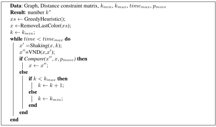
The overall VNS algorithm is shown in Figure 1. The algorithm inputs the following
data: distance constraint matrix, valueskminandkmax, denoting the minimal and
maxi-mal neighborhood structures,timemax- maximal allowed execution time and the value
pmove, representing the probability of shifting from one solution to another, in a case of
equal objective functions. After the data input, VNS starts with a greedy heuristic
(de-scribed in Subsection 3.1), which gives the upper bound (U B) for the total number of
colors. After theU B is determined, the initial value ofk∗ is set toU B (legal coloring
withU B colors), and the starting solution of the VNS is constructed by the procedure
Init(). Initial solution uses one color less than the value U B. This procedure, together
with the objective function, is described in Subsection 3.2. The minimization process is performed in the shaking procedure (Subsection 3.3) and the VND procedure, which is, together with the Compare procedure described in Subsection 3.4. During the minimiza-tion process inside the VND procedure the algorithm is trying to improve the soluminimiza-tion to the feasible one. If this situation happens, the valuek∗is decreased by one, that legal col-oring is remembered and the algorithm repeats the search process by decreasing the total number of colors. The algorithm stops when the maximum execution time is reached. The result of the algorithm is the valuek∗, i.e. thek∗-coloring of the given graph.
Data: Graph, Distance constraint matrix,kmin,kmax,timemax,pmove Result: numberk∗
xs←GreedyHeuristic();
x←RemoveLastColor(xs);
k←kmin;
whiletime < timemaxdo
x0=Shaking(x, k);
x00=VND(x,x0);
ifCompare(x00, x, pmove)then
x←x00; else
ifk < kmaxthen
k←k+ 1;
else
k←kmin;
end end end
3.1. Constructive heuristics
Before the minimization process is started, an initial solution (legalk-coloring, for some
k) needs to be constructed. Our algorithm uses the greedy approach similar to the greedy
algorithm used and minutely described in [19,7]. This greedy algorithm takes a sequence of ’split nodes’, greedily assigning colors to them. For each node a set of ’forbidden’ colors is first formed and after that the algorithm chooses the smallest color not belonging to that set.
In the literature, other approaches for getting starting solutions are also used. For example, Malaguti and Toth in [20], considered several greedy algorithms proposed for solving VCP: sequential greedy algorithm (SEQ), as well as another greedy approach -DSATUR from [2], similar to SEQ, but one which dynamically chooses the vertex to color next, i.e. the one which minimizes a given score. In order to fast compute an initial upper bound, Malaguti and Toth performed 20 runs of the greedy algorithm SEQ.
Malaguti and Toth’s greedy approach in most case instances achieves better (lower) upper bounds than the greedy algorithm we took from [7], but the experiments indicate that presented VNS easily decrease those (higher) upper bounds. Therefore, using slightly greater starting values ofkcould not significantly aggravate the overall optimization pro-cess. The exceptions of this “rule” can appear in some cases of small instances, where Malaguti and Toth’s greedy algorithm achieves nearly best known solutions, so iteration process needs to decrease the upper bound only for few values. In these cases, our algo-rithm needs some more time, since it starts with higher upper bounds.
In recent papers ([15,16,14]), the proposed algorithms simply start with the best known value ofkfrom the literature as a starting value and try to construct the feasiblek-coloring. In case of success, i.e. the legalk-coloring is found, the algorithms decrease the valuek
by 1 and try to find thek−1coloring. This iterative process stops when no legal coloring can be found. Although this approach appears to be very successful and can speed up the overall process (because the algorithms do not spend any time to construct some starting solution and decrease it many times in the optimization process), we still decided to fol-low the approach used in [19,20,7]: our basic approach is to construct an initial feasible solution by greedy algorithm and improve it in the iteration process, while the stopping criteria are not satisfied.
3.2. The initialization and the objective function
For the given graphG= (V, E), the solution is represented by an integer array of the
di-mensionn, n=|V|. After the upper bound (U B) is determined by the greedy approach,
For the given solutionx, represented by the array (x1, x2, ..., xn), wherexi, i =
1..nis the color assigned to the vertexi, the objective function Calculate() is defined as follows:
Calculate(x) = X
{i,j}∈E
max{0, d(i, j)− |xi−xj|}, (1)
whered(i, j)is the given distance between the verticesi andj. From the equation (1) it can be seen that the infeasible solutions are penalized by increasing the value of the objective function, if the distance conflicts appear. In a case when there are no distance conflicts, the objective function is equal to 0 and in that case the solution is feasible i.e. the legal coloring is found. Additionally to the calculating the objective function, in the
procedure Calculate() for each vertexvwe remember the valueconf licts(v)containing
the value of distance conflicts ofv. More precisely, this value is calculated by the formula:
conf licts(v) = X
j:{v,j}∈E
max{0, d(v, j)− |xv−xj|}. (2)
These values, obtained for each vertexv ∈V, take places for the arrangement of the
vertices, performed inside the VND procedure.
3.3. Neighborhoods and Shaking procedure
The shaking procedure creates a new solutionx0,x0 ∈ Nk(x), which is based on the
current best solutionx.
In order to define the k-th neighborhood we use the following procedure. Somek
vertices fromV are chosen randomly and for each chosen vertex, the color is randomly
changed to some other color from the interval[1, max color], wheremax color is the
maximal color used in the coloring. The solutionx0, formed in the described way is the
subject of the further improvements in the VND.
In the algorithm, the valuekmin is set to 2. Experiments show that the algorithm
achieves best performances forkmax= 20.
3.4. Variable neighborhood descent
After the solutionx0 is obtained by the shaking procedure, a series of special designed
(ncis total number of used colors) are harder to be replaced by another, comparing to the
colors far off-the middle. So, if two verticesuandvhave the same number of conflicts,
conf licts(u) =conf licts(v), we first chooseuif|nc/2−xu|<|nc/2−xv|, otherwise
we first choosev.
In order to further improve the behaviour of the VND, we involve one additional cri-terion for the arrangement of the vertices, in cases when first two criteria do not make any difference between vertices. The third criterion is based on two components: for
each vertexvwe calculate the valueweights(v), as the sum of the weights (distances)
of the edges incident with v. Additionally, for the vertex v, we take into account the
maximal edge weight (distance) for the vertex v (maxw(v)). Finally, the third
crite-rion is calculated by the geometric mean of these two values, i.e. in cases when first
two criteria do not determine the priority, the vertex uis chosen before the vertex v if
p
weights(u)·maxw(u)>pweights(v)·maxw(v). Otherwise, the VND first choose
v. Although the third criterion influence on the ordering relatively rarely, the experiments show that it refines the ordering of vertices in a good direction and improves the overall VND.
Beside the main experiments described in Subsections 4.1 and 4.2, in order to justify the usage of these three criteria, additional experiments are performed. In the experiments (described in Subsection 4.3), various combinations of the mentioned criteria are consid-ered. The obtained results indicate that the approach of using all three criteria generally provides better results than variants in which some of these criteria are omitted.
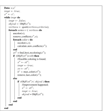
The pseudocode of the VND procedure is shown in Figure 2.
After the objective function for the solutionx00is calculated by the function ObjF() and the array of vertices is arranged by using the mentioned criteria, the VND iteratively chooses the vertices from that array. For the selected vertexv, the VND is trying to find “better” color in the following way. If the vertexvis currently colored by the colorxv,
we first “uncolor” that vertex, also removing the conflicts which arise by using that color for the vertexv. It should be noted that we do not need to calculate the objective function from the beginning, since only conflicts related to the chosen vertex influence on the total
sum. Therefore, after only these conflicts are removed, we iteratively color the vertexv
by all other colors, trying to find better coloring. Simultaneously, we calculate the new conflicts, which appear by new coloring and remember these values (conflicts). After we tried all the colors for the vertexv, we choose the one, which generates the least total sum of conflicts. In that way, we get a new temporary solutionxt00and three possibilities can happen:
– The objective value ofxt00 is equal to 0: That means that the VND was totally
suc-cessful and not just improved the objective value, but gave the feasible coloring with the less number of colors than the previous best one. In this case, we remember that coloring, setxs=xt00and continue the search as follows: we set up a new current so-lutionx00=xt00and replace the maximal color inx00by some other, randomly chosen color. The VND, i.e. the improvement process is then applied again on the currentx00
and the next vertex. It should be noted that if this case happen, the maximum number of colors may be decreased by more than one in one such step.
– The objective value ofxt00 is greater than 0, but still less than the starting one: we
hold the changes arisen in the current step, we setx00=xt00and continue the VND
Data:x,x0
impr←true;
x00←x0; whileimprdo
impr←f alse;
objval←ObjF(x00);
vertices←qsort(vertices,criteria); foreachvertexv∈verticesdo
uncolor(v);
remove conflicts(x00,v); foreachcolorcdo
recolor(v,c);
calculate new conflicts(x00); end
xt00= find best recoloring(x00); if (ObjF(xt00)==0)then
//feasible coloring is found;
x00←xt00;
impr←true;
xs←xt00;
k∗←max color(xt00); remove last color(x00); else
if (ObjF(xt00)< objval)then //improvement happened;
x00←xt00;
impr←true;
objval= ObjF(xt00); end
end end end
– The objective value ofxt00is greater or equal than the starting one: we continue the
VND withx00and the next vertex, without any change.
The VND finishes when no more improvements can be done and the algorithm analysis the results of the VND in the procedure Compare: In cases when number of colors used in the solutionx00is less than in the solutionx, or if the objective value ofx00is less than of thex, the currently best solution xgets the valuex00. If the objective values of the two solutionsxandx00are the same, thenx=x00is set with probabilitypmoveand the
algorithm continues the search with the same neighborhood. In all other cases, the search
is repeated with the samexand the next neighborhood.
Because of the fact that there can be a large number of solutions with the same ob-jective value in a neighbor of the current best one (especially when the obob-jective value is decreased to 1), the decision whether the algorithm will move or not to another so-lution of the same quality is very important step. Therefore, appropriate setting the pa-rameterpmove, which influence to that decision is a crucial part for success of the overall
searching process. Although some VNS implementations allow low values ofpmove, even
pmove= 0(see for example [23]), the experiments indicate that the proposed algorithm
for solving BCP achieves best performances for the value pmove = 0.5. While in the
case of BCP lower values of parameter pmove usually leads to premature convergence
into suboptimal solutions, higher values should also be avoided, since they can cause the
appearance of cycles. The valuepmove= 0.5is a compromise between these two extreme
cases, since it gives enough probability to move to another solution of the same quality, while the probability of the appearance of the cycle is still rather low.
4.
Experimental results
This section presents the experimental results, which show the effectiveness of the pro-posed VNS. All the tests are carried out on the Intel i7-4770 CPU @3.40 GHz with 8 GB RAM and Windows 7 operating system. For each execution, only one thread/processor is used. The VNS is implemented in C programming language and compiled with Visual Studio 2010 compiler.
For all experiments we used standard set of GEOM instances, which consists of 33 geometric graphs generated by Michael Trick, available in [33]. In each GEOM instance, points are generated in a 10,000 by 10,000 grid and are connected by an edge if they are close enough together. Edge weights are inversely proportional to the distance between vertices, which simulates the real situations where closer adjacent vertices stronger inter-ference each other. This set contains three types of graphs: for each dimension, one sparse (GEOMn) and two denser graphs (GEOMna and GEOMnb) are given. The instances are originally generated for BCP, but they are also transformed for solving BMCP, by in-troducing the weights of vertices. For BMCP, vertex weights are uniformly randomly generated, between 1 and 10 for sets GEOMn and GEOMna, and between 1 and 3 for set GEOMnb.
CPU, we used a standard benchmark program (dfmax), together with a benchmark in-stance (R500.5) also used in the reference works. For this inin-stance, we report the comput-ing time of 8 seconds, which is similar to the times reported in other recent works. Similar to the approach in [16], we set the timeout limits to 2 hours for BCP instances and 4 hours for MBCP instances. The algorithm stops if it cannot solve the coloring within the time limit. For each instance, we performed 30 independent executions, which is also the case in [15].
4.1. Experimental results on BCP instances
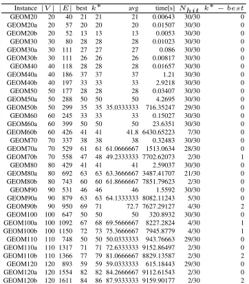
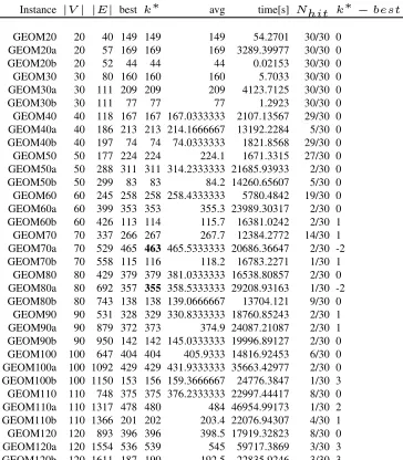
This section reports the experimental results obtained on the first set of instances, related to BCP problem. Table 1 provides the results obtained by the presented VNS. The data in the table are organized as follows: first three columns contain the instance name, number of vertices (|V|) and number of edges (|E|). The fourth column contain the best known result from the literature. The next five columns contain data related to the VNS: column (k∗) contains the best found result, the average result (columnavg) obtained in 30 runs, the total average execution time in seconds needed to achieve the presented best result (columntime), the hit rate (Nhit), as well as the column (k∗−best), which contains
the difference between the best result obtained by the VNS and the previous best-known result from the literature.
Table 1.Results of the VNS obtained on BCP instances
Instance|V| |E|bestk∗ avg time[s]Nhit k∗ −best
GEOM20 20 40 21 21 21 0.00643 30/30 0
GEOM20a 20 57 20 20 20 0.01507 30/30 0
GEOM20b 20 52 13 13 13 0.0053 30/30 0
GEOM30 30 80 28 28 28 0.01023 30/30 0
GEOM30a 30 111 27 27 27 0.086 30/30 0
GEOM30b 30 111 26 26 26 0.00817 30/30 0
GEOM40 40 118 28 28 28 0.01657 30/30 0
GEOM40a 40 186 37 37 37 1.21 30/30 0
GEOM40b 40 197 33 33 33 2.9218 30/30 0
GEOM50 50 177 28 28 28 0.03407 30/30 0
GEOM50a 50 288 50 50 50 4.2695 30/30 0
GEOM50b 50 299 35 35 35.0333333 716.35247 29/30 0
GEOM60 60 245 33 33 33 0.15027 30/30 0
GEOM60a 60 399 50 50 50 23.6351 30/30 0
GEOM60b 60 426 41 41 41.8 6430.65223 7/30 0
GEOM70 70 337 38 38 38 0.32483 30/30 0
GEOM70a 70 529 61 61 61.0666667 1513.0634 28/30 0 GEOM70b 70 558 47 48 49.2333333 7702.62073 2/30 1
GEOM80 80 429 41 41 41 2.59037 30/30 0
GEOM80a 80 692 63 63 63.3666667 3487.41707 21/30 0 GEOM80b 80 743 60 60 61.8666667 7851.79623 2/30 0
GEOM90 90 531 46 46 46 1.5592 30/30 0
GEOM90a 90 879 63 63 64.1333333 8082.11243 5/30 0
GEOM90b 90 950 69 71 72.7 7627.29127 4/30 2
GEOM100 100 647 50 50 50 320.8932 30/30 0
GEOM100a 100 1092 67 68 69.5666667 8227.2824 4/30 1 GEOM100b 100 1150 72 73 75.3666667 7945.8779 4/30 1 GEOM110 110 748 50 50 50.0333333 943.76663 29/30 0 GEOM110a 110 1317 71 71 72.6333333 9152.86497 2/30 0 GEOM110b 110 1366 77 79 81.0666667 8829.13587 2/30 2 GEOM120 120 893 59 59 59.0333333 615.18443 29/30 0 GEOM120a 120 1554 82 82 84.2666667 9112.61543 2/30 0 GEOM120b 120 1611 84 86 87.9333333 9159.90177 2/30 2
GEOM20, GEOM30, GEOM40 instances, which are equal to 21, 28 and 28, respectively. From Table 1, it can be seen that the proposed VNS algorithm achieves all best known results for smaller instances up to 60 vertices.
For the rest of the instances (total of 18 middle and larger instances), VNS achieves 12 best results and in 6 out of 18 cases VNS is not able to reach previously best-known solution from the literature.
The proposed VNS solves the sparse graphs (GEOMn) easier than the dense ones
(GEOMna and GEOMnb). From the columnNhit, it can bee seen that the ratio between
the number of runs of the VNS when the previously best-known solution is reached and the total number of runs (30) is rather high for sparse graphs.
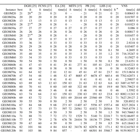
Table 2 describes the comparison of our approach to the state-of-the-art methods. The data are organized as follows: The first column contain the instance name. The rest of the table contain data related to the approaches: the best result of the Discropt general heuris-tics (DGH) presented by Phan and Skiena [25] (the execution time is not reported), Prest-wich’s forward checking coloration neighborhood search (FCNS) from [27], Malaguti and Toth’s evolutionary algorithm (EA) from [20], the MITS algorithm presented by Lai and Lu from [15], path relinking (PR) algorithm from [16] and learning hybrid-based search (LHS) from [14]. All these results are extracted from [14]. Last three columns contain best results, the execution times for the proposed VNS and the difference between best VNS and previous best known result. It should be noted that the execution times are very
different and are not reasonable comparable, since the algorithms achieve differentk
-colorings and the algorithms were run on the machines with different CPU speeds.
Table 2.Comparison of the proposed VNS algorithm to other reference works on BCP instances
DGH [25] FCNS [27] EA [20] MITS [15] PR [16] LHS [14] VNS Instance best k ktime[s] time[s] ktime[s] ktime[s] ktime[s]k∗ time[s] diff
GEOM20 21 20∗ 21 0 21 0 - - 21 0 21 0 21 0.00643 0
GEOM20a 20 20 20 0 20 0 20 0 20 0 20 0 20 0.01507 0
GEOM20b 13 13 13 0 13 0 13 0 13 0 13 0 13 0.0053 0
GEOM30 28 27∗ 28 0 28 0 - - 28 0 28 0 28 0.01023 0
GEOM30a 27 27 27 0 27 0 27 0 27 0 27 0 27 0.086 0
GEOM30b 26 26 26 0 26 0 26 0 26 0 26 0 26 0.00817 0
GEOM40 28 27∗ 28 0 28 0 - - 28 0 28 0 28 0.01657 0
GEOM40a 37 38 37 0 37 0 37 0 37 0 37 0 37 1.21 0
GEOM40b 33 36 33 0 33 0 33 0 33 0 33 0 33 2.9218 0
GEOM50 28 29 28 0 28 0 28 0 28 0 28 0 28 0.03407 0
GEOM50a 50 54 50 2 50 0 50 0 50 0 50 0.1 50 4.2695 0
GEOM50b 35 40 35 0 35 0 35 3 35 1 35 1.2 35 716.35247 0
GEOM60 33 34 33 0 33 0 33 0 33 0 33 0 33 0.15027 0
GEOM60a 50 54 50 1 50 0 50 1 50 0 50 0.1 50 23.6351 0
GEOM60b 41 47 43 0 41 29 41 277 41 105 41 214.7 41 6430.65223 0
GEOM70 38 40 38 0 38 0 38 0 38 0 38 0 38 0.32483 0
GEOM70a 61 64 62 2 61 12 61 45 61 47 61 23.7 61 1513.0634 0 GEOM70b 47 54 48 1 48 52 47 8685 47 6678 47 665.4 48 7702.62073 1
GEOM80 41 44 41 0 41 0 41 0 41 0 41 0.1 41 2.59037 0
GEOM80a 63 69 63 12 63 150 63 21 63 12 63 6.6 63 3487.41707 0 GEOM80b 60 70 61 0 60 145 60 322 60 191 60 19.9 60 7851.79623 0
GEOM90 46 48 46 3 46 0 46 0 46 0 46 0 46 1.5592 0
GEOM90a 63 74 64 2 63 150 63 230 63 191 63 23.8 63 8082.11243 0 GEOM90b 69 83 72 2 70 1031 69 20144 69 23560 69 779.2 71 7627.29127 2
GEOM100 50 55 50 0 50 2 50 2 50 2 50 1 50 320.8932 0
GEOM100a 67 84 68 9 68 273 67 11407 67 5556 67 1557.4 68 8227.2824 1 GEOM100b 71 87 73 15 73 597 72 24561 72 41832 71 2038.6 73 7945.8779 2
GEOM110 50 59 50 4 50 3 50 2 50 5 50 1.3 50 943.76663 0
GEOM110a 71 88 73 7 72 171 72 1529 71 5140 71 2218.7 71 9152.86497 0 GEOM110b 77 87 79 2 78 676 78 24416 78 18136 77 2598.7 79 8829.13587 2
GEOM120 59 67 60 4 59 0 59 1 59 2 59 0.5 59 615.18443 0
GEOM120a 82 101 84 4 84 614 82 34176 82 62876 82 171.1 82 9112.61543 0 GEOM120b 84 103 86 9 84 857 - - 85 66301 84 3568.7 86 9159.90177 2
achieved by older methods from [25] and [27] are improved by the newer ones. According to [6], the results of three instances GEOM20, GEOM30 and GEOM40 reported in [25] are probably wrong, so they are marked with the asterisk symbol. The VNS and EA from [20] give 28 same best results, in 3 cases EA is better and VNS is better in two cases. Comparing to the MITS from [15], for VNS and MITS 23 equal best results are reported, in 5 cases MITS is better, in one case VNS is better. In four cases, no solution is reported in [15]. VNS achieve 27 same solutions as the two most recent methods PR and LHS, and in 6 cases PR and LHS are better than VNS.
4.2. Experimental results on BMCP instances
Algorithm developed for BCP instances can also be applied for solving BMCP, after the implicit transformation of each BMCP to BCP instance. From the experimental results presented in this section we see that our VNS achieve many previously known best known results and two new best ones.
Table 3 provides the results obtained on BMCP instances. Table 3 is organized similar to the case of BCP instances: first four columns contain the instance name, number of vertices (|V|) and number of edges (|E|) and the best known result from the literature. The
next five columns contain data related to the VNS: column (k∗) contains the best found
result, the average result (columnavg) obtained in 30 runs, the total average execution
time in seconds needed to achieve the presented best result (columntime), the hit rate
(Nhit), as well as the column (k∗−best), which contains the difference between the best
result obtained by the VNS and the previous best-known result from the literature. In columnk∗, new best results are marked in bold.
Table 3.Results of the VNS obtained on BMCP instances
Instance|V| |E|bestk∗ avg time[s]Nhit k∗ −best
GEOM20 20 40 149 149 149 54.2701 30/30 0 GEOM20a 20 57 169 169 169 3289.39977 30/30 0
GEOM20b 20 52 44 44 44 0.02153 30/30 0
GEOM30 30 80 160 160 160 5.7033 30/30 0 GEOM30a 30 111 209 209 209 4123.7125 30/30 0
GEOM30b 30 111 77 77 77 1.2923 30/30 0
GEOM40 40 118 167 167 167.0333333 2107.13567 29/30 0 GEOM40a 40 186 213 213 214.1666667 13192.2284 5/30 0 GEOM40b 40 197 74 74 74.0333333 1821.8568 29/30 0 GEOM50 50 177 224 224 224.1 1671.3315 27/30 0 GEOM50a 50 288 311 311 314.2333333 21685.93933 2/30 0 GEOM50b 50 299 83 83 84.2 14260.65607 5/30 0 GEOM60 60 245 258 258 258.4333333 5780.4842 19/30 0 GEOM60a 60 399 353 353 355.3 23989.30317 2/30 0 GEOM60b 60 426 113 114 115.7 16381.0242 2/30 1 GEOM70 70 337 266 267 267.7 12384.2772 14/30 1 GEOM70a 70 529 465463465.5333333 20686.36647 2/30 -2 GEOM70b 70 558 115 116 118.2 16783.2271 1/30 1
GEOM80 80 429 379 379 381.0333333 16538.80857 2/30 0 GEOM80a 80 692 357355358.5333333 29208.93163 1/30 -2 GEOM80b 80 743 138 138 139.0666667 13704.121 9/30 0
Data in Table 3 indicate that VNS achieves 21 best known results and in 2 cases VNS obtains new best results. In 10 cases, VNS could achieve results close to the best ones. For all smaller BMCP instances (up to 50 vertices), VNS obtains all previous best-known results, with a relatively high hit rate for most of them. VNS achieves 2 new best results, for two middle instances GEOM70a and GEOM80a. For 9 large-sized instances, (100-120 vertices), VNS achieves previously known best results in 4 cases and in 5 cases VNS achieves nearly best results.
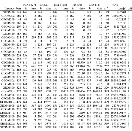
Table 4 shows the comparative results obtained by the state-of-the-art methods from the literature and the proposed VNS. The first column of the table contains the instance name. The next five blocks of two columns contain best results and execution times of the five recent and most successful methods from the literature: FCNS [27] by Prestwich, Malaguti and Toth’s EA from [20], the MITS algorithm from [15] presented by Lai and Lu, path relinking (PR) algorithm from [16] and learning hybrid-based search (LHS) from [14]. Like in the case of BCP, all these results are also extracted from [14]. Last three columns contain best results, the execution times for the proposed VNS and the difference between best VNS and previous best-known results.
Table 4.Comparison of the proposed VNS algorithm to other reference works on BMCP instances
FCNS [27] EA [20] MITS [15] PR [16] LHS [14] VNS Instance best k time k time k time k time k timek∗ time[s] diff GEOM20 149 149 4 149 18 149 2 149 1 149 1.8 149 54.2701 0 GEOM20a 169 170 2 169 9 169 15 169 7 169 0.5 169 3289.39977 0
GEOM20b 44 44 0 44 5 44 0 44 0 44 0 44 0.02153 0
GEOM30 160 160 0 160 1 160 0 160 0 160 0.1 160 5.7033 0
GEOM30a 209 214 11 210 954 209 10 209 26 209 16.2 209 4123.7125 0
GEOM30b 77 77 0 77 0 77 0 77 0 77 0 77 1.2923 0
GEOM40 167 167 1 167 20 167 0 167 1 167 0.2 167 2107.13567 0 GEOM40a 213 217 299 214 393 213 328 213 133 213 9 213 13192.2284 0
GEOM40b 74 74 4 74 1 74 2 74 4 74 1.5 74 1821.8568 0
GEOM50 224 224 1 224 1197 224 8 224 2 224 0.3 224 1671.3315 0 GEOM50a 311 323 51 316 4675 314 40373 312 270860 311 1452.6 311 21685.93933 0 GEOM50b 83 86 1 83 197 83 1200 83 723 83 72.1 83 14260.65607 0 GEOM60 258 258 77 258 139 258 19 258 23 258 1.3 258 5780.4842 0 GEOM60a 353 373 10 357 8706 356 38570 354 34580 353 9007.1 353 23989.30317 0 GEOM60b 113 116 12 115 460 113 104711 113 63579 113 910.7 114 16381.0242 1 GEOM70 266 277 641 272 1413 270 7602 266 130844 266 2534 267 12384.2772 1 GEOM70a 465 482 315 473 988 467 38759 466 6952 465 36604.946320686.36647 -2 GEOM70b 115 119 55 117 897 116 213545 116 26110 115 3640.7 116 16783.2271 1
GEOM80 379 398 361 388 132 381 212213 380 34493 379 357.8 379 16538.80857 0 GEOM80a 357 380 109 363 8583 361 41235 358 41772 357 4340335529208.93163 -2 GEOM80b 138 141 37 141 1856 139 255 138 705 138 46.5 138 13704.121 0 GEOM90 328 339 44 332 4160 330 4022 328 134941 328 162.2 329 18760.85243 1 GEOM90a 372 382 13 382 5334 375 10427 372 282456 372 16782.1 373 24087.21087 1 GEOM90b 142 147 303 144 1750 144 211366 144 14648 142 7680.8 142 19996.89127 0 GEOM100 404 424 7 410 3283 404 40121 404 16355 404 64.9 404 14816.92453 0 GEOM100a 429 461 26 444 12526 442 381 436 9108 429 78363.1 429 35663.42977 0 GEOM100b 153 159 367 156 3699 156 213949 156 86308 153 10840.1 156 24776.3847 3 GEOM110 375 392 43 383 2344 381 183 375 25401 375 1598.8 375 22997.44417 0 GEOM110a 478 500 29 490 2318 488 926 482 9819 478 49457.1 480 46954.99173 2 GEOM110b 201 208 5 206 480 204 944 201 47653 201 5388.4 202 22076.94307 1 GEOM120 396 417 9 396 2867 - - 396 15341 396 626.1 396 17919.32823 0 GEOM120a 536 565 41 559 3873 554 1018 539 45147 536 69518.6 539 59717.3869 3 GEOM120b 187 196 3 191 3292 189 213989 189 14371 187 8025.8 190 22835.9246 3
From Table 4 it can be seen that FCNS, EA, MITS and PR could achieve most of the best known solutions for small instances up to 50 vertices, and LHS and VNS achieve all of the best known solutions for small instances. MITS and PR fails to achieve best known solution only for one small instance (GEOM50a).
of instances, PR could achieve 6 best known solutions and in other cases is close to the best ones. LHS achieves all best known solutions except in ten cases and in two cases close to the best ones. VNS achieves five best known solutions, in five cases VNS achieve solutions close to the best ones and in two cases VNS finds new best solutions.
For the large-size instances, FCNS could not find any best known solution, while EA and MITS achieve only one best known solution. PR achieves four best known solutions and for other large-size instances achieve solutions relatively close to the best ones. While LHS achieves all best knows solutions for large instances, VNS achieve best ones for six instances and for the rest nearly best solutions.
Regarding execution times, it is obvious that they are quite different, since different
approaches provide results with differentkvalues. Additionally, some of the algorithms
(like EA and VNS) spend additional time for the construction phase, while other algo-rithms (MITS, PR and LHS) start with the previous best known solutions.
4.3. Justification of the usage of the criteria in the VND procedure
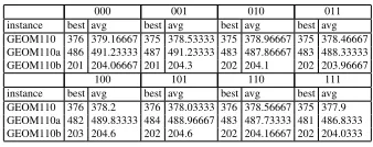
In order to further analyse the behaviour of the proposed VND procedure and to justify the usage of the criteria for ordering vertices, additional experiments are performed with three large BMCP instances (namely GEOM110, GEOM110a and GEOM110b). Recall that in the VND procedure three criteria are combined for determining the ordering: the first criterium is the total number of conflicts for the vertex, the second is the distance of the color assigned to the vertex from the middle and the third one is the geometric mean of the total sum of the weights of the edges incident with the vertex and the maximal edge distance for that vertex. In the experiment, total of eight possible different variants of the overall criterium are analysed: each of the mentioned three criteria is or is not used.
Table 5 provides the experimental results obtained in all of these eight cases. Each case is denoted asXY Z, whereX, Y andZbelongs to{0,1}, indicating if the criterium is used (value 1) or not used (value 0). For each case, best found and average results are shown. The time limit for this experiment is set to 3000s. From Table 5, it can be seen
Table 5.Comparison of the various combinations of the criteria used in the VND
000 001 010 011
instance best avg best avg best avg best avg GEOM110 376 379.16667 375 378.53333 375 378.96667 375 378.46667 GEOM110a 486 491.23333 487 491.23333 483 487.86667 483 488.33333 GEOM110b 201 204.06667 201 204.3 202 204.1 202 203.96667
100 101 110 111
instance best avg best avg best avg best avg GEOM110 376 378.2 376 378.03333 376 378.56667 375 377.9 GEOM110a 482 489.83333 484 488.96667 483 487.73333 481 486.8333 GEOM110b 203 204.6 202 204.6 202 204.16667 202 204.0333
achieves better best result than the proposed one, but the average value obtained by the proposed variant is better.
These results indicate that the usage of the proposed combination of the criteria is justified, having in mind that some other variants can also reach high quality results.
5.
Conclusions
In this paper we present the VNS algorithm for solving two generalizations of the vertex coloring problems: bandwidth coloring problem and multiple bandwidth coloring prob-lem. Since BCP and MBCP enjoy many applications, presented algorithm and achieved results are of a great interest for both theory and practice.
In the shaking procedure, an increasing number of vertices are permuted, forming the new solution which is subject of the further improvement in the VND. In the VND proce-dure, vertices are arranged in a way to increase the probability of successful recoloring. This approach of the arrangement of the vertices splits the local search in a series of dis-joint procedures, enabling better choices of the vertices which are addressed to re-color. The overall criterion for the ordering the vertices is based on the number of conflicts of each vertex, combined with two additional criteria.
The algorithm is tested on the common used instances. In the case of BCP, VNS achieves many previous best-known results and in the case of BMCP, VNS obtains two new best solutions in a reasonable time. Experimental results indicate that the proposed VNS becomes one of state-of-the-art methods for solving BCP and BMCP.
The further investigation of this problem can include parallelization and running on some powerful multiprocessor system, as well as the application of the proposed method for solving some similar real-life problems.
References
1. Aardal, K., Hoesel, S., Koster, A., Mannino, C., Sassano, A.: Models and solution techniques for frequency assignment problems. Annals of Operations Research 153(1), 79–129 (2007) 2. Br´elaz, D.: New methods to color the vertices of a graph. Commun. ACM 22(4), 251–256 (Apr
1979)
3. Budiono, T., Wong, K.W.: A pure graph coloring constructive heuristic in timetabling. In: Com-puter Information Science (ICCIS), 2012 International Conference on. vol. 1, pp. 307–312 (June 2012)
4. Burke, E.K., McCollum, B., Meisels, A., Petrovic, S., Qu, R.: A graph-based hyper-heuristic for educational timetabling problems. European Journal of Operational Research 176(1), 177 – 192 (2007)
5. Chiarandini, M., St¨utzle, T.: Stochastic local search algorithms for graph set t-colouring and frequency assignment. Constraints 12(3), 371–403 (2007)
6. Diasa, B., de Freitasa, R., Maculanc, N., Michelond, P.: Solving the bandwidth coloring prob-lem applying constraint and integer programming techniques
7. Fijuljanin, J.: Two genetic algorithms for the bandwidth multicoloring problem. Yugoslav Jour-nal of Operations Research 22(2), 225–246 (2012)
9. Hale, W.: Frequency assignment: Theory and applications. Proceedings of the IEEE 68(12), 1497–1514 (Dec 1980)
10. Hansen, P., Mladenovi´c, N.: Variable neighborhood search. Springer (2005)
11. Hern´andez-P´erez, H., Rodr´ıguez-Mart´ın, I., Salazar-Gonz´alez, J.J.: A hybrid grasp/vnd heuris-tic for the one-commodity pickup-and-delivery traveling salesman problem. Computers & Op-erations Research 36(5), 1639 – 1645 (2009), selected papers presented at the Tenth Interna-tional Symposium on LocaInterna-tional Decisions (ISOLDE X)
12. Hertz, A., Mittaz, M.: A variable neighborhood descent algorithm for the undirected capaci-tated arc routing problem. Transportation Science 35(4), 425–434 (2001)
13. Hu, B., Raidl, G.R.: Variable neighborhood descent with self-adaptive neighborhood-ordering. In: Proceedings of the 7th EU/MEeting on Adaptive, Self-Adaptive, and Multi-Level Meta-heuristics. Citeseer (2006)
14. Jin, Y., Hao, J.K.: Effective learning-based hybrid search for bandwidth coloring. IEEE Trans-actions on Systems, Man, and Cybernetics: Systems 45(4), 624–635 (2015)
15. Lai, X., Lu, Z.: Multistart iterated tabu search for bandwidth coloring problem. Computers & Operations Research 40(5), 1401 – 1409 (2013)
16. Lai, X., Lu, Z., Hao, J.K., Glover, F., Xu, L.: Path relinking for bandwidth coloring problem. arXiv preprint arXiv:1409.0973 (2014)
17. Lewis, R., Thompson, J., Mumford, C., Gillard, J.: A wide-ranging computational comparison of high-performance graph colouring algorithms. Computers & Operations Research 39(9), 1933 – 1950 (2012)
18. Lim, A., Zhang, X., Zhu, Y.: A hybrid methods for the graph coloring and its related problems. In: Proceedings of MIC2003: The Fifth Metaheuristic International Conference. Kyoto, Japan (2003)
19. Lim, A., Zhu, Y., Lou, Q., Rodrigues, B.: Heuristic methods for graph coloring problems. In: Proceedings of the 2005 ACM Symposium on Applied Computing. pp. 933–939. SAC ’05, ACM, New York, NY, USA (2005)
20. Malaguti, E., Toth, P.: An evolutionary approach for bandwidth multicoloring problems. Euro-pean Journal of Operational Research 189(3), 638 – 651 (2008)
21. Malaguti, E., Toth, P.: A survey on vertex coloring problems. International Transactions in Operational Research 17(1), 1–34 (2010)
22. Marti, R., Gortazar, F., Duarte, A.: Heuristics for the bandwidth colouring problem. Int. J. Metaheuristics 1(1), 11–29 (May 2010)
23. Matic, D.: A variable neighborhood search approach for solving the maximum set splitting problem. Serdica Journal of Computing 6(4), 369–384 (2012)
24. Mladenovi´c, N., Hansen, P.: Variable neighbourhood search. Computers & Operations Re-search 24, 1097–1100 (1997)
25. Phan, V., Skiena, S.: Coloring graphs with a general heuristic search engine. In: Computational Symposium on Graph Coloring and its Generalization. pp. 92–99 (2002)
26. Prestwich, S.: Constrained bandwidth multicoloration neighbourhoods. In: Computational Symposium on Graph Coloring and its Generalization. pp. 126–133 (2002)
27. Prestwich, S.: Generalised graph colouring by a hybrid of local search and constraint program-ming. Discrete Applied Mathematics 156(2), 148 – 158 (2008)
28. Qu, R., Burke, E.K., McCollum, B.: Adaptive automated construction of hybrid heuristics for exam timetabling and graph colouring problems. European Journal of Operational Research 198(2), 392 – 404 (2009)
29. Roberts, F.S.: T-colorings of graphs: recent results and open problems. Discrete Mathematics 93(23), 229 – 245 (1991)
30. Sabar, N., Ayob, M., Qu, R., Kendall, G.: A graph coloring constructive hyper-heuristic for examination timetabling problems. Applied Intelligence 37(1), 1–11 (2012)
32. Tesman, B.A.: Set t-colorings. Congressus Numerantium 77, 229–242 (1990)
33. Trick, M.: Computational symposium: Graph coloring and its generalizations, http://mat.gsia.cmu.edu/color02/ (2002),http://mat.gsia.cmu.edu/COLOR02/
Dragan Mati´creceived his BSc (2001) and MSc (2009) degrees in mathematics at the Faculty of Mathematics and Natural Sciences, University of Novi Sad, Serbia and PhD degree (2013) in Mathematics at the Faculty of Mathematics at the University of Bel-grade, Serbia. His research interests in science include combinatorial optimization and metaheuristics, and their application in various fields of mathematics, computer science, industry and education.
Jozef Kraticawas born in 1966 in Belgrade, Serbia. He received his B.Sc. degrees in mathematics (1988) and computer science (1988), M.Sc. in mathematics (1994) and Ph.D. in computer science (2000) from University of Belgrade, Faculty of Mathematics. In 2002 he joined Mathematical Institute as a researcher. As a delegation leader participated on the International Olympiads in Informatics (IOI’90 Minsk - Belarus, IOI’93 Mendoza - Argentina). His research interests include genetic algorithms (evolutionary computa-tion), variable neighborhood search, electromagnetism-like metaheuristic, optimization on graphs and location problems.
Vladimir Filipovi´cis associate professor at the Faculty of Mathematics, University of Belgrade, Serbia. He received his PhD degree in Computer Science at the Faculty of Mathematics, University of Belgrade (2006).His research interests include combinato-rial optimization, operational research, computational intelligence, metaheuristics and big data. He supervised four PhD theses.