https://doi.org/10.5194/nhess-17-1683-2017 © Author(s) 2017. This work is distributed under the Creative Commons Attribution 3.0 License.
Multi-variable flood damage modelling with limited data using
supervised learning approaches
Dennis Wagenaar, Jurjen de Jong, and Laurens M. Bouwer Deltares, Boussinesqweg 1, 2629 HV, Delft, the Netherlands
Correspondence to:Dennis Wagenaar ([email protected]) Received: 4 January 2017 – Discussion started: 12 January 2017
Revised: 25 July 2017 – Accepted: 30 July 2017 – Published: 29 September 2017
Abstract. Flood damage assessment is usually done with damage curves only dependent on the water depth. Sev-eral recent studies have shown that supervised learning tech-niques applied to a multi-variable data set can produce signif-icantly better flood damage estimates. However, creating and applying a multi-variable flood damage model requires an extensive data set, which is rarely available, and this is cur-rently holding back the widespread application of these tech-niques. In this paper we enrich a data set of residential build-ing and contents damage from the Meuse flood of 1993 in the Netherlands, to make it suitable for multi-variable flood damage assessment. Results from 2-D flood simulations are used to add information on flow velocity, flood duration and the return period to the data set, and cadastre data are used to add information on building characteristics. Next, several statistical approaches are used to create multi-variable flood damage models, including regression trees, bagging regres-sion trees, random forest, and a Bayesian network. Validation on data points from a test set shows that the enriched data set in combination with the supervised learning techniques de-livers a 20 % reduction in the mean absolute error, compared to a simple model only based on the water depth, despite sev-eral limitations of the enriched data set. We find that with our data set, the tree-based methods perform better than the Bayesian network.
1 Introduction
Decision making in flood risk management is increasingly based on studies that quantify the flood risk rather than only the flood hazard. Flood damage estimation is therefore be-coming increasingly important (Merz et al., 2010). Flood
risk assessment supports policy makers in deciding which flood risk management measures are most efficient in reduc-ing flood risks and how much investment is cost efficient. With the European Union Floods Directive (EC, 2007) now fully in place, national flood risk assessments are being de-veloped with the final aim to support flood risk management plans. In the Netherlands, such flood damage assessment has been used to derive the optimal protection standard for flood protection (Kind, 2013; van der Most, 2014), using the cur-rent Dutch standard method for damage modelling (Kok et al., 2005). Also, for insurance applications, more precise es-timates of flood damage are required.
Flood risk assessments require flood damage models. These models typically predict the damage as fraction of the potential damage, based on the water depth, and average building repair and replacement costs for different types of buildings (Messner et al., 2007; Jonkman et al., 2008). Sim-ilar approaches are also applied to other natural hazards, for example for landslides (Papathoma-Köhle et al., 2015), and the software package HAZUS can be used for floods, earth-quakes and hurricanes (Scawthorn et al., 2006). Alternative approaches to calculate flood risk also exist, such as vulner-ability indicators (Papathoma-Köhle, 2016).
(Wa-genaar et al., 2016). This can cause errors, as simple models hold many implicit assumptions that may not be valid for the situation the model is transferred to. For instance, Elmer et al. (2010) showed that an event with a low flood probabil-ity could not use the same damage function as a flood event with a high probability. These implicit assumptions cause large unexplained differences between flood damage func-tions (Wagenaar et al., 2016; Gerl et al., 2016). However, transferability can be improved when a model describes more variations of the damaging process, and when more variables are included in the damage models (e.g. flood probability is explicitly part of the model). Similar problems are also present in the modelling of other natural hazards. For exam-ple, Fuchs et al. (2007) found that building materials are very important for debris flow damage modelling and that models can therefore not always be transferred in space and time.
Current approaches suffer from two main limitations: first, they rely on limited information and usually only take into account water depth as a predictor, and use a determinis-tic relation between water depth and some fraction of av-erage maximum damages; second, they are deterministic in nature, while it has been shown that uncertainties in this approach are large, but generally not quantified (e.g. in the Dutch standard method; Egorova et al., 2008). Some of the multi-variable methods are able to provide probability distri-butions, rather than deterministic estimates of damage.
Recently, multi-variable flood damage models have been created with a German data set based on telephone inter-views. Thieken et al. (2005) found that apart from the water depth also the contamination of the flood water and precau-tionary measures were important to estimate the flood dam-age. In Thieken et al. (2008) these extra variables were in-cluded in a simple multi-variable flood damage model as a surcharge. Using information from this same database, Merz et al. (2013) used regression and bagging trees and Vogel et al. (2014) used Bayesian networks to predict the flood dam-age. Spekkers et al. (2014) applied regression trees to esti-mate pluvial flood damage. Van Oostegem et al. (2015) ap-plied the Tobit estimation technique to a multi-dimensional data set in Belgium to estimate pluvial flood damages. These multi-variable flood damage models have been shown to per-form better than simple flood damage models by Schröter et al. (2014) (up to 25 % reduction in mean absolute error, MAE), both tested on their own data set and on data sets from other floods (Schröter et al., 2014). Also, some multi-variable approaches (Bayesian networks, bagging trees and random forests) generate probability distributions of estimated dam-age, and thus provide information on uncertainties of the es-timates. Therefore, multi-variable flood damage models look like a promising approach to improve flood damage mod-elling.
The application of multi-variable flood damage models for flood risk management studies is still difficult because of the large data requirements. Running a multi-variable flood dam-age model for a new area requires for every object several
variables on the flood hazard and building characteristics that are not yet typically collected. Creating new multi-variable flood damage models is currently rarely done because they also require records of flood damage at building level.
More commonly available (although still rare) are simple data sets that hold records with the flood damage that oc-curred for each building with sometimes a few other vari-ables (such as location or water depth). Such data sets may have been created for compensation purposes or to build sim-ple flood damage models but may miss most of the desired variables. An example of such a data set is the flood dam-age data set collected after the Meuse flood of 1993 in the Netherlands which is used here. Previously this data set has been described in Wind et al. (1999) and in more detail in WL Delft (1994). In this paper we explore the use of supervised learning techniques to build flood damage models based on a data set that is very different from the data sets used in pre-vious studies (i.e. the German data set applied by Merz et al., 2013, and Schröter et al., 2014). The data set in this pa-per was collected by insurance expa-perts directly after the flood for compensation purposes and covers all affected buildings. This is different from the German data set, which was col-lected a year after the flood for research purposes based on a sample of the affected buildings. The data are also differ-ent in that in the original study only a few variables were collected, in contrast to the German data set, where all vari-ables (except return period) were based on telephone inter-view answers. In this study several methods are applied to enrich the Meuse 1993 flood damage data set with extra flood hazard and building characteristic variables. We will answer the question of whether this enriched data set from a differ-ent source than previous studies is also suitable to build a multi-variable flood damage model. The expectation is that a multi-variable model performs better than a model based on a single variable (water depth) and that even data with limited quality will improve the results.
2 Methods and data 2.1 Data sets
2.1.1 Meuse 1993 damage data set
The data set available for this research is based on the Meuse flood of 22 December 1993 in the province of Limburg in the Netherlands (WL Delft, 1994). Although no dike breaches occurred in this event, several towns and urban areas lo-cated close to the river were affected. The flood caused a total of 254 million guilder (price level 1993) in direct dam-ages, which is approximately EUR 180 million today (price level 2016). The flood inundated 180 km2, which is about 8 % of the province of Limburg. Some 32 % of the damage pertains to residential buildings and content (furnishings). In this study only residential damage is considered. Other major damage categories were business (29 %), government (24 %) and agriculture (8 %) (WL Delft, 1994). These categories are not considered because they are more heterogeneous and fewer data about them are available.
Damage information was collected in the context of a com-pensation arrangement for flood damage by the national gov-ernment. All data were collected by sending damage experts from insurance companies to the affected buildings, several weeks after the flood event had occurred. Directly after the damage data were collected in 1994, the data were shared with WL Delft (now Deltares) to create a flood damage model. WL Delft received 5780 records for damage to resi-dential buildings. The damage to privately owned resiresi-dential buildings was collected by an organization called “Sticht-ing Watersnood 1993”. The damage to companies and the structure of rental residential buildings was collected by an-other organization called “Stichting Watersnood Bedrijven 1993”. Therefore, in this set-up of damage data collection, the building structure information of rental residential build-ings was collected by “Stichting Watersnood Bedrijven”, the organization that collected data on company damages. This is different from the organization that collected the rest of the residential damage information. The data on structural dam-age to rental residential buildings was only shared with WL Delft (1994) in a partial aggregated form. WL Delft (1994) presumably distributed this partially aggregated rental resi-dential building damage data over the individual rental res-idential buildings. The exact method for this was, however, not reported and the original data set is no longer available. Therefore, we had to work with a data set which includes un-known manual actions. The structure damage data are there-fore of inconsistent quality; the content damage, however, has no such problems. Furthermore, it is believed that the percentage of rental residential buildings in the affected area of Limburg is relatively low, limiting the impact of this data problem.
Another issue with the data set is that for privacy reasons the exact locations of the buildings were not shared with
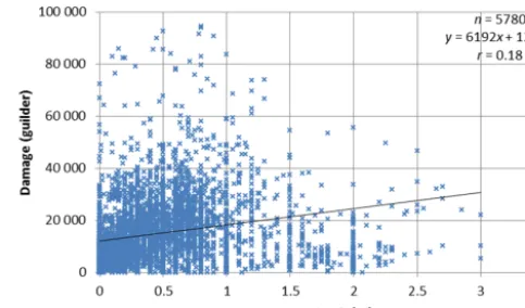
Figure 1.Scatter plot showing the relation between water depth and damage in the original data set.
WL Delft. Only the six-digit postal code was available for this study, which makes it difficult to enrich the data set, as between 1 and 20 buildings share the same six-digit postal codes in the data set.
In the original data set the water depth (relative to the ground floor level) was estimated by the experts that sur-veyed the damage. The quality of the water depth estimate is questioned by WL Delft (1994; report 9) because it was not the main aim of the survey and the experts visited several weeks after the water had receded. A plot of the water depth (see Fig. 1) and the damage does not show an obvious rela-tion. The correlation between the water depth and the damage is weak (Pearson correlation coefficient=0.18).
The final data set also contains information on the number of inhabitants per building, whether the house has a base-ment and whether the house was attached to other houses. However, these data are not described in any of the avail-able reports so the collection methods are not known, but the recorded values are clear enough to incorporate in this study. Two more variables are also included in the WL Delft data set and also not described in any available report. These are emergency actions and ownership of the house. The mean-ing of the values found in the data set for these variables is, however, not sufficiently clear, and could unfortunately not be taken into account in this study.
2.1.2 Upgraded Meuse 1993 database
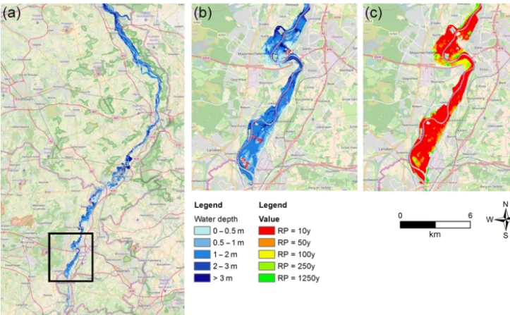
Figure 2. (a)Simulated water depth for the entire study area in Limburg.(b)Simulated water depth and affected population (in red) for an example area.(c)The return period at which areas start flooding for the example area. The example area is defined in the box in the left picture. The scale bar corresponds to the example area.
variables. Using this model, a new simulation was run using a discharge boundary condition at Eijsden and a water level boundary condition at Keizersveer for the period 1 November 1993 to 31 January 1994. This simulation was used to create a maximum water depth map, a flood duration map, a flood return period and a flow velocity map at a spatial resolution varying between 10 and 40 m.
The maximum water depth and flow velocity are standard outputs of WAQUA. Flood duration is, however, not a stan-dard output and is more difficult to obtain from a 2-D flood simulation because the drainage also needs to be included in the schematization (Wagenaar, 2012). During the 1993 Meuse flood, most drainage occurred because of the natural slope in terrain and therefore the 2-D flood simulation im-plicitly includes most of the drainage because the discretized bed level is included. The flood duration can then be calcu-lated by analysing the time-varying maps of the water depth and calculating for every cell the time between the moment a cell is inundated and the moment the cell is dry again. How-ever, some cells in the digital elevation map in WAQUA are surrounded by cells that have a higher elevation. These cells do not drain in the 2-D flood simulation and are still inun-dated at the end of the simulation. For these cells the flood duration has been calculated based on the change in water depth. If the water depth in a cell stays the same in the sim-ulation for 24 subsequent hours the cell is considered dry at the moment this stable water depth is first reached.
Simulations were also run with the same Meuse 1993 schematization for design discharges with 1, 10, 50, 100, 250 and 1250 return periods. These discharges are based on
HR2006 (Diermanse, 2004) and have discharges of respec-tively 1300, 2260, 2869, 3109, 3431 and 4000 m3s−1. The results of these simulations were combined to create a flood return period map for the Meuse 1993 situation. This map shows for each cell at what return period it first floods. Fig-ure 2 shows that large water depths occurred and that most of the area floods frequently. The majority of the houses are, however, located in the safest areas with the lowest water depths and highest return periods.
These maps (water depth, flow velocity, flood duration and return periods) were linked to the original damage records using cadastre data. The data of the cadastre have exact build-ing locations, postal codes, livbuild-ing area within the residen-tial buildings, the building footprint area and the construc-tion year. The building year was used to filter the data to find the building stock of 1993. Then, based on the building lo-cations, the 2-D flood simulation results were linked to the cadastre data.
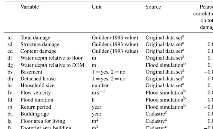
Ta-Table 1.Description of the variables in the flood damage data set for the Meuse flood of 1993.
Variable Unit Source Pearson
correlation on total damage
td Total damage Guilder (1993 value) Original data seta 1
sd Structure damage Guilder (1993 value) Original data seta 0.85 cd Content damage Guilder (1993 value) Original data seta 0.83
df Water depth relative to floor m Original data seta 0.18
dg Water depth relative to DEM m Flood simulationb 0.18
bs Basement 1=yes, 2=no Original data seta −0.04
dh Detached house 1=yes, 2=no Original data seta 0.08
hs Household size number Original data seta 0.17
fv Flow velocity m s−1 Flood simulationb 0.04
fd Flood duration h Flood simulationb 0.05
rp Return period year Flood simulationb −0.09
ba Building age year Cadastrec 0.01
la Floor area for living m2 Cadastrec 0.04
fa Footprint area building m2 Cadastrec −0.02
aWL Delft, 1994.b2-D flood simulation data using WAQUA.cBasisregistraties Adressen en Gebouwen (BAG), version 2011 (Kadaster: https://www.kadaster.nl/bag).
ble 1 gives an overview of the available records in this com-bined data set.
The method of joining cadastre objects with damage records within a postal code area based on water depth rank is error prone. The modelled water depth is on average 30 cm larger than the recorded water depth. This is possibly because of the difference in reference level of both data sources, as the recorded water depth is relative to the floor level and the modelled water depth is relative to the digital elevation map. Not all houses have the same floor elevation and both the recorded and the modelled water depth are uncertain because of recording and model imprecisions. It is therefore likely that some damage records have been linked to the wrong ob-ject. However, errors will likely be limited because the join on postal codes is accurate. Object and flood variables are generally similar for buildings within the same postal code area (e.g. houses within a street are typically similar to each other), so these errors are expected not to significantly dis-turb the general trends in the data. The errors are therefore considered acceptable given that the purpose of the data set is only to build a flood damage model. If significant errors are present this would result in a reduced performance of the supervised learning algorithms on the test set. A relatively simple alternative to this water depth rank method is also ap-plied. In this alternative, the average value at all building lo-cations in the postal code area was assigned to each of the objects in the postal code.
2.2 Supervised learning algorithms
Several supervised learning techniques have been applied to the enriched data set to build multi-variable flood damage
models. The different supervised learning techniques all have different ways to generalize the training data in such a way as to give useful predictions of the total damage.
These multi-variable flood damage models are compared to two different reference models to assess the value of the enriched data set and to assess the value of multi-variable flood damage models in general. In what follows, the differ-ent supervised learning algorithms applied are described in further detail.
2.2.1 Regression: root function
The first reference model only uses the square root of the water depth (see Eq. 1) to predict the flood damage. This model represents the damage functions commonly applied today in flood risk management studies because many dam-age functions have approximately the shape of a root function (e.g. Scawthorn et al., 2006; Thieken et al., 2008; Penning-Rowsell et al., 2005; Sluijs et al., 2000). Merz et al. (2012) applied the same method to get a reference damage function. The purpose of this reference model is to see the benefits of using more data.
The root function (1) is fitted to the data set in such a way that the coefficientsc1andc2are optimized to get the small-est possible error based on the total damage (td) and water depth (wdf) data. The values of the coefficients are optimized for the best fit with the ordinary least-squares method. This is done with the Python package SciPy:
td=c1+c2 √
2.2.2 Multi-variable linear regression
The second reference model uses multi-variable linear re-gression to fit a linear model to the data. This model repre-sents simpler/traditional techniques to make a multi-variable model from data. The purpose of this reference model is to see the benefits of potentially better techniques to build multi-variable models from data. Multi-variable linear re-gression is for example used in Islam (1997) to make multi-variable flood damage models. Linear regression is used without transformations of the input variables because there is no clear indication in the data that there are non-linear re-lationships (for example see Fig. 1).
To ensure that the model captures general trends and does not fit too strongly to the observed data (overfitting) the LASSO technique is used. This technique determines the co-efficients in such a way that a penalty is applied for increas-ing the coefficients and usincreas-ing the variables more. LASSO yields sparse models, so some coefficients will become zero, which means they are not useful for the prediction. There-fore, the LASSO technique is useful for variable selection. To make this work correctly the data are normalized before training the model.
The multi-variable linear regression was carried out with the Scikit learn library in Python (Pedregosa et al., 2011). LASSO requires an alpha parameter to be set which deter-mines the height of the penalty applied. Several alpha values were tried (0, 0.5, 1 and 10). The model is very insensitive to the alpha value (all formulations perform about equally well); an alpha value of zero performed best on all indica-tors. Therefore, it was not optimized further and the alpha is set to zero. When alpha is zero the method is equal to the or-dinary least-squares method and no overfitting prevention is in place and LASSO is not necessary. This shows that over-fitting is not an issue for relatively simple techniques such as linear regression with this data set and number of variables.
2.2.3 Regression tree learning
Decision trees are a way to represent complex relationships between data and classes in a tree structure. A decision tree can be seen as a series of binary questions (nodes) leading to an answer in the form of a class (leaf). A question can be related to any variable at any value (e.g. is the water depth smaller than 0.5 m).
A regression tree is similar to decision trees but instead of classes it results in real numbers. In theory, regression trees can be very large and have a separate leaf for each unique value in the data set. However, it is more common to com-bine several similar unique values inside the same leaf and represent it with a summary statistic number (mean). In such a case the regression tree is an approximation of the relation-ship.
Regression tree learning algorithms can create optimal re-gression trees based on a data set. In this paper the data set
consists of 4398 flood damage records (incomplete records are discarded) with 11 variables for each damage record (see Table 1). The regression tree algorithm aims to split the data set into subsets in such a way that the mean squared error (MSE) of the predicted total damage for all observations is minimized compared to the observed data. It does this by calculating the reduction for all candidate splitting variables according to their value and then picking the combination that maximizes the MSE reduction (1I )– this is shown in Eq. (2), wheren is the total number of observations in the node,yn is the vector of observed target values in the node andy is the mean of the target values in the node.ynL and ynR are vectors with the observed target values of the left and right group after the split andyL andyRare the mean observed target value for the left and the right group. The re-gression tree is grown by repeating this process at each node of the tree. This has been done with the Scikit learn library in Python (Pedregosa et al., 2011):
1I= 1 n
X
(yn−y)2− X
ynL−yL 2
−X(ynR−yR)2
. (2)
(Pedregosa et al., 2011). Accordingly, the results shown do not include pruning.
2.2.4 Bagging regression trees
Another method to avoid overfitting and generally improve the accuracy of decision/regression trees is bootstrap aggre-gating, also called bagging. The idea behind the method is to resample the data set multiple times and to build a new regression tree for each resampled data set. This results in an ensemble of regression trees. The resulting flood damage is then the average of the ensemble of regression trees. Re-sampling is done by building several data sets by randomly picking records from the original data set (each record is al-lowed to be used multiple times in the same data set). Every resampled data set therefore randomly leaves out a fraction of the observations and puts more weight on other observations because they are picked multiple times. Bagging regression trees also lead to probabilistic outcomes because the ensem-ble of trees can be seen as a probability distribution of the outcome.
2.2.5 Random forest
A random forest is a more advanced variation of bagging gression trees. Apart from building multiple trees with re-sampled data sets it also randomly excludes a subset of vari-ables at each decision split. This will result in an ensemble of regression trees each based on a different set of damage records and each leaving out a different number of variables at each decision split. For this paper the default settings of Scikit learn are applied. In our case this means that eight vari-ables are left out at each decision split.
2.2.6 Bayesian network
A Bayesian network is a type of probabilistic graphical model that represents a set of random variables and their conditional dependences in a directed acyclic graph (DAG) structure. Each variable in the network may be observed or represented as a prior probability distribution and de-pendences between variables are represented with edges representing joint probability distributions. The edges in a Bayesian network are directed, which means there is a direc-tion in which the influence of one variable flows to the other. From this network, inference can be used in order to utilize knowledge of one variable to make predictions about other variables.
Bayesian networks and probabilistic graphical models in general are used in many different fields, such as bioinfor-matics (e.g. Mourad et al., 2011), image processing (e.g. Sudderth and Freeman, 2008) and speech recognition (e.g. Bilmes, 2002). Recently, they have also been applied to flood damage modelling (Vogel et al., 2014; Schröter et al., 2014; Van Verseveld, 2014). Schröter et al. (2014) found that their performance is often better than that of the different types of
tree methods. Furthermore, a Bayesian network can give its result as a probability distribution and does not require infor-mation about each variable in order to make predictions. If fewer variables are available, the Bayesian network handles this by adjusting the probability distribution of the outcome. This makes it ideal for transfer of models to other locations where fewer data are available than for the location where the model was originally based. Furthermore, it returns (for each object) probability distributions rather than deterministic val-ues, which is valuable for assessing uncertainties within the damage model estimates.
A Bayesian network can be discrete, continuous or a com-bination. In this paper fully discrete Bayesian networks are used, in which all variables are discretized into bins. Given a network, the probability of a particular set of discrete vari-able values can be calculated with the following formula:
P (Xi, . . ., Xn)= n
Y
i=1
P (Xi|parents(Xi)) , (3)
whereXi are the variables and parents(Xi)is the set of
vari-ables directed to Xi. The probability of a single variable
value can be obtained by taking the sum of all the proba-bilities that contain the variable value of interest. The con-ditional probabilities are stored in concon-ditional probability ta-bles (CPTs). These tata-bles show, for each combination of par-ent variable values, the probability of each possible output value.
A data-driven Bayesian network can derive all its CPTs from the data and even derive its graph structure from the data. For this paper, two Bayesian networks were con-structed: a data-driven Bayesian network with both the graph structure and the CPTs derived from the data set and an ex-pert network in which the graph structure was estimated in an expert session but the CPTs were derived from the data set. All calculations were done with a Python library called libpgm (Cabot, 2012). This library follows the methodology described in Koller and Friedman (2009).
Discretization was achieved by splitting the data into bins with an equal number of data points in each bin. This works better than making equal-sized bins because of the large extremes in, especially, the damage data. Equal-sized bins would either increase the number of bins, which is detrimen-tal to the maximum likelihood estimation (having bins that contain no observations), or the bins would be so large that a majority of the data points would end up in the same bin, which would limit the Bayesian network performance. The number of bins per variable was chosen based on the per-formance of a test set on the MAE criterion. This was done by varying the discretization of the most important variables until the smallest error was found. For the Bayesian network with the data-driven structure the number of bins chosen was slightly larger because the network is less complex than the expert network.
The performance of the Bayesian network on the testing data can be sensitive for discretization. There are two possi-ble alternatives for the discretization method applied in this paper: an optimization algorithm could be applied to deter-mine the optimal discretization, or a continuous Bayesian network could be used (Friedman and Goldszmidt, 1996). Apart from solving the discretization problem the advantage of a continuous Bayesian network is that it would probably perform better in predicting extreme values but a disadvan-tage is that the Bayesian network is restricted to specific fam-ilies of parametric probability distributions (Friedman and Goldszmidt, 1996). An optimization algorithm for the dis-cretization can minimize the error produced by the discretiz-ing but does not solve the fundamental problem of havdiscretiz-ing too few data points.
The data-driven structure is also learned with the libpgm Python library. This library is using a constraint-based ap-proach for structure learning, as is described in Koller and Friedman (2009). In a constraint-based approach the struc-ture is learned by calculating dependences and conditional dependences between the variables. When two variables are dependent regardless of what they are conditioned by, an edge (connection) is formed. The algorithm follows this pro-cedure to create the entire network. The result is shown in Fig. 4a.
As an alternative to the data-driven structure a struc-ture was also made in an expert meeting involving sev-eral Deltares flood damage/Bayesian network experts (see acknowledgements). In the expert meeting the network was constructed based on a combination of expert judge-ment/logic and with the knowledge of Fig. 3 in this paper. The experts focused mainly on edges that they thought were relevant for estimating the flood damage. The result is shown in Fig. 4b.
The relationship between the total, structural and con-tents damage is known and not probabilistic: total dam-age=structure damage+contents damage. Also, in our case the structure damage, contents damage and total damage are always dependent variables. Therefore, using a Bayesian
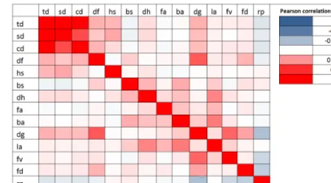
net-Figure 3.Correlation coefficients between the different variables. See Table 1 for a description of the abbreviations.
Figure 4.Bayesian network learned from data(a)and Bayesian network constructed by experts(b). Note that not all variables are used in the network.
work to model this exact definitional relationship could only introduce extra errors and not add any extra explanation. Therefore in the expert network it was decided not to use the total damage variable. Instead the total damage is calcu-lated as the sum of the expected value of the structure and the contents damage. In the data-driven network the struc-ture damage was not included by the algorithm. Therefore, the total damage variable itself is used for the data-driven network.
not the case (for the expert model) – the MAE is even slightly worse when calculated on its own data (0.622), the correla-tion coefficient andR2are only slightly better (0.24 and 0.04) and only the mean bias error (MBE) is significantly better (−0.015). See results section for comparison.
2.3 Variable importance
In order to investigate the value of more data it is interest-ing to study the contribution of the different variables to the prediction accuracy. This can be done with bagging trees and the random forest methods. This importance can be calcu-lated as the (normalized) total reduction of the mean square error brought by the different variables as achieved during the training of the models. This can be used to compare the relative importance of the variables between each other. This feature importance can be calculated for all the regression trees in the ensemble and a general importance is computed by the Scikit learn library by taking the average of the feature importances in the tree. This was applied in this study for the bagging trees. The variable importance has been separated for predicting the importance of the total damage, structural damage and the content damage. For the calculation of the variable importance the data set is used in which the average per postal code is used for the new variables. The water depth rank is not used because it could transfer some of the impor-tance of the original water depth value to the new variables.
Another way to study variable importance is with the LASSO technique in multi-variable linear regression. LASSO can drop unimportant variable coefficients to zero. If a variable is dropped to zero it means that the variable is less important.
3 Results
3.1 Model comparison
The different models were tested on a test set that was not used for training the models. Four indicators are used to rate the performance of the models: MAE, MBE, the Pearson cor-relation coefficient and the coefficient of determination (R2). The MAE indicator is the mean absolute error divided by the average damage, so a smaller MAE is a better model. The MBE indicator is the average error; this differs from the MAE in that an overestimation is able to correct for an under-estimation and vice versa. A low MBE shows that the sum of a large number of predictions will probably be very accurate. The Pearson correlation coefficient is a measure of the linear dependence between two variables. This measure is used to compare the predicted damage with the actual damage in the test set. A Pearson correlation of 1 means a perfect correla-tion, 0 means no correlation and−1 means a perfect inverse correlation. R2 is the predictive capacity of a model com-pared to just using the average damage as a prediction. If the R2is 0 it means that the independent variables add no
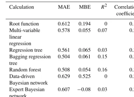
predic-Table 2. Results of different models for four indicators: MAE, MBE,R2and correlation coefficient. The models had access to all variables (except for the root function). The version of the data set with the water depth rank join between the old and the new variables is used.
Calculation MAE MBE R2 Correlation
coefficient
Root function 0.612 0.194 0 0.15
Multi-variable 0.578 0.055 0.07 0.27
linear regression
Regression tree 0.561 0.065 0.03 0.31
Bagging regression 0.504 0.061 0.15 0.38 tree
Random forest 0.508 0.054 0.16 0.39
Data-driven 0.629 0.525 0 0.21
Bayesian network
Expert Bayesian 0.607 −0.08 0.03 0.21 network
tive capacity compared to just using the average. WhenR2is 1 it means that the independent variables can explain all vari-ation in the dependent variable. Table 2 shows the results for the different models.
Table 2 shows that given that the models can use all data, random forest and bagging regression trees perform best and equally well. These two methods reduce the MAE by 12 % compared to a reference model using the same data (multi-variable linear regression). Bagging regression trees and ran-dom forest perform significantly better than normal regres-sion trees, as was also noted by Merz et al. (2013) for flood damage in Germany. Random forest and bagging regression trees also outperform the Bayesian networks. The normal re-gression tree also works better than the Bayesian networks. This contradicts the findings of Schröter et al. (2014), that in most cases Bayesian networks outperformed the regression trees. Schröter et al. (2014), however, had a very different data set from the one applied in this study.
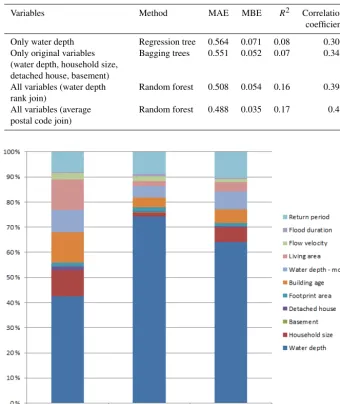
Table 3.The best-performing model based on the MAE indicator with different number of variables.
Variables Method MAE MBE R2 Correlation
coefficient
Only water depth Regression tree 0.564 0.071 0.08 0.306
Only original variables (water depth, household size, detached house, basement)
Bagging trees 0.551 0.052 0.07 0.345
All variables (water depth rank join)
Random forest 0.508 0.054 0.16 0.394
All variables (average postal code join)
Random forest 0.488 0.035 0.17 0.41
Figure 5.Variable importance: the contribution of different variables in reducing the error in the bagging regression trees (the chart follows the order of the legend).
Some wrong observations may then have a relatively large impact on the damage prediction.
In the data-driven network the variable of interest (total damage) in our test is only influenced by the water depth. This is because the water depth relative to the ground floor is known while the content damage is not known, so the known water depth blocks all the influence of other variables and the unknown content damage has no influence because it is unknown (it is a target variable). The data-driven Bayesian network is therefore in our test in practice only dependent on the water depth. Hence, the structure learning decides to ig-nore the other variables when the water depth relative to the ground floor is available. This is probably because the data-driven structure algorithm finds all variables equally impor-tant and therefore draws only the most imporimpor-tant edges
(con-nections) regarding the total damage. Other methods (e.g. as described by Riggelsen, 2008) for structure learning might be able to give better results.
3.2 Benefits of more data
The models were trained with different numbers of variables to see whether the additional data are valuable. As expected, the best-performing model with a high number of variables always performs significantly better than the best-performing model with fewer variables (see Table 3). More data therefore seem to add potential value to the damage prediction despite the possible quality issues in the additional data. The MAE of the best-performing model with only the water depth (regres-sion tree) can be reduced by a further 14 % by the best model using all data (random forest). The MAE of the root func-tion fitted to the data (representing common practice) can be reduced by about 20 % using the random forest with all data. The method to join the extra data with the original data based on water depth rank is not effective. Just taking the av-erage value per postal code appears to work better. The water depth rank probably sometimes assigns extreme variable val-ues to the wrong objects which disturbs some correlations in the data.
3.3 Variable importance
The total importance of variables that were added in this study is about 30 % (Fig. 5), which means that 30 % of the er-ror reduction during the training of bagging tree model orig-inates from variables that were added to the data set. The added variables therefore clearly help to improve the predic-tion accuracy. This assessment was done without the water depth ranking join because this could assign some of the im-portance of the original water depth to the modelled water depth. The original water depth is by far the most important variable. Construction year is an important variable for the structure damage but not for content damage. This is as ex-pected. Household size is quite important for the structural damage but insignificant for the content damage. This is less obvious, but it could be that large families live on average in larger houses but do not have much more valuable con-tents on the ground floor. Return period is an important vari-able for both the structure and the content damage. This was also expected because the population in areas that flood more frequently are expected to have more flood experience, thus resulting in better preparedness and therefore less damage. This effect is visible in the data, with return period having an importance of about 10 %.
For the best-fitting multi-variable linear regression model (LASSO alpha=0) no variables are dropped. Only when al-pha is increased to 10 are five variables dropped; however, this also causes a slight drop in model performance (MAE goes from 0.578 to 0.588). The dropped variables are build-ing footprint, buildbuild-ing age, livbuild-ing area, flood duration and flow velocity. Of these dropped variables, two have a signif-icant importance in the bagging tree variable importance as-sessment. These are building age and living area. It could be that these variables are more important in non-linear models.
4 Discussion and conclusion
Additional data improve flood damage modelling relative to a test set, even if these data come from a collection of dif-ferent sources and are of limited quality (error prone). The supervised learning algorithm is also important. Given the same data there are large differences between the algorithms. Random forests and bagging regression trees perform signif-icantly better than normal regression trees and multi-variable linear regression. The Bayesian networks perform poorly compared to any of the tree-based methods.
Our current approach does not show that the additional variables are beneficial for the Bayesian networks. However, because the tree methods can benefit from the additional data it is likely that in some cases Bayesian networks could also. The poor performance of the Bayesian networks contradicts earlier studies (Schröter et al., 2014) and could be due to the discretization method, quality of the expert network, network learning algorithm or problems with data quantity or quality. The test set that was applied in this paper for the valida-tion of the model was randomly selected from the data and consistently applied among all models. The accuracy of the indicators for model performance could perhaps be further improved through some form of cross-validation. Also, the tweaking of different models could become more accurate if cross-validation was used instead of validation on a single test set only. For example, the optimization of the stop crite-ria for tree-based models and the alpha value in the LASSO method for the multi-variable linear regression could be im-proved in that way. Expectations are that this would cause minor improvements in results but that it would not influence the conclusions of this paper.
This paper did not address another benefit of Bayesian net-works, random forest and bagging trees, which is the incor-poration of uncertainty. Bayesian networks do this explicitly in the method and for bagging trees or random forest each tree can be seen as a possible damage estimate, and together the trees represent a probability distribution.
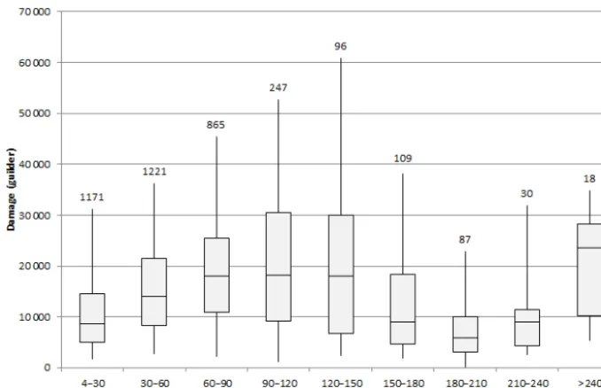
Figure 6.Box plots of the Meuse flood of 1993 per water depth class. The box shows the 25–75 % interval and the lines show the 5–95 % interval. The line in the middle of the box shows the median value. The labels on top of the plots show the number of observations per water depth class.
of preferring Bayesian networks over tree-based methods in the future.
The data set applied in this paper had many limitations. The most important limitation is that the exact locations of the objects are unknown. Because of this, it was difficult to link building and flood characteristics to damage records. An attempt to do this by using water depth rank performed worse than just using the average variable values per postal code. Despite this limitation, the added data still produced signif-icantly better damage estimates. Another problem with the data set is the unknown manual adjustment to an unknown share of data (rental residential buildings) for the structural damage records. These actions may have introduced a rela-tionship between structural damage and some of the origi-nally recorded variables that was not there in reality. This could in theory cause a slight overestimation in the predic-tion performance of the models on the test set. This effect on the results is, however, expected to be small because most of the prediction improvements came from adding variables that were not available for doing the manual actions in 1994. This study applied absolute damages rather than relative damages. This requires the supervised learning algorithms to implicitly also predict information about the values at risk be-sides the vulnerability. The algorithms can do this with vari-ables such as living area, footprint area, building year and household size. This seems less error prone and better than estimating such values at risk with general rules of thumb based on assumptions about construction costs and content value. Such assumptions could cause extra errors, and there-fore in this study absolute damages were used.
Supervised learning can help to create and improve flood damage models. They have many theoretical advantages over deterministic damage functions based on only water depth. The application of supervised learning in flood damage mod-elling remains challenging in practice because of limited data availability. In this paper we utilized different data sources compared to previous studies to acquire these data and showed that also on this data set the methods are ben-eficial, especially the tree-based methods. Future work may merge available data sets from different events and from dif-ferent countries in order to develop a model that can be ap-plied using several hazard variables, and which also works in circumstances outside areas for which flood damage data are available.
Data availability. The dataset “Observed flood damages from the 1993 Meuse flood in the Netherlands with added flood and building characteristics” is given in the supplement below.
The Supplement related to this article is available online at https://doi.org/10.5194/nhess-17-1683-2017-supplement.
Competing interests. The authors declare that they have no conflict of interest.
Special issue statement. This article is part of the special issue “Damage of natural hazards: assessment and mitigation”. It is a re-sult of the EGU General Assembly 2016, Vienna, Austria, 17–22 April 2016.
Acknowledgements. We thank our colleagues Kathryn Roscoe for advice on the Bayesian networks and our colleagues Karin de Bruijn and Marcel van der Doef for their input in constructing the expert Bayesian network. We would also like to thank the editor (Thomas Thaler) and the reviewers (one anonymous reviewer and Sven Fuchs) – their detailed constructive comments and sugges-tions helped to substantially improve this paper. This research has received funding from the European Union’s Horizon 2020 research and innovation programme under grant agreement number 641811 (Improving predictions and management of hydrological extremes – IMPREX); see also http://www.imprex.eu.
Edited by: Thomas Thaler
Reviewed by: Sven Fuchs and one anonymous referee
References
Becker, A.: Maas-modellen 5de generatie: Modelopzet, kalibratie en verificatie, Deltares rapport 1204280-000-ZWS-0011, 2012 (in Dutch).
Bilmes, J.: Graphical models and automatic speech recognition, J. Acoust. Soc. Am., 112, 2278, https://doi.org/10.1121/1.4779134, 2002.
Breiman, L., Friedman, J., Olshen, R. A., and Stone, C. J.: CART: Classification and Regression Trees, Wadsworth, Belmont, CA, 1984.
Cabot, C.: Libpgm Python library, pythonhosted.org/libpgm, avail-able at: http://pythonhosted.org/libpgm/, (last access: 10 Au-gust 2016), 2012.
Diermanse, F. L. M.: HR2006 – herberekening werklijn Maas, Delft Hydraulics Q3623.00, 2004 (in Dutch).
EC: DIRECTIVE 2007/60/EC of the European Parliament andof the Council of 23 October 2007 on the assessment and manage-ment of flood risks, Official Journal of the European Union, L 288/27, 2007
Egorova, R., van Noortwijk, J., and Holterman, S.: Uncertainty in flood damage estimation, International Journal River Basin Man-agement, 6, 139–148, 2008.
Elmer, F., Thieken, A. H., Pech, I., and Kreibich, H.: Influence of flood frequency on residential building losses, Nat. Hazards Earth Syst. Sci., 10, 2145–2159, https://doi.org/10.5194/nhess-10-2145-2010, 2010.
Friedman, N. and Goldszmidt, M.: Discretizing continuous at-tributes while learning bayesian networks, In Proc. ICML, 157– 165, 1996.
Fuchs, S., Heiss, K., and Hübl, J.: Towards an empirical vulnera-bility function for use in debris flow risk assessment, Nat. Haz-ards Earth Syst. Sci., 7, 495–506, https://doi.org/10.5194/nhess-7-495-2007, 2007.
Gerl, T., Kreibich., H, Franco, G., Marechal, D., and Schröter, K.: A Review of Flood Loss Models as Basis for Har-monization and Benchmarking, PLoS ONE, 11, e0159791, https://doi.org/10.1371/journal.pone.0159791, 2016.
Islam, K. M. N.: The impacts of flooding and methods of assessment in urban areas of Bangladesh, PhD Thesis, Middlesex University, 1997.
Jongman, B., Kreibich, H., Apel, H., Barredo, J. I., Bates, P. D., Feyen, L., Gericke, A., Neal, J., Aerts, J. C. J. H., and Ward, P. J.: Comparative flood damage model assessment: towards a Eu-ropean approach, Nat. Hazards Earth Syst. Sci., 12, 3733–3752, https://doi.org/10.5194/nhess-12-3733-2012, 2012.
Jonkman, S. N., Bockarjova, M., Kok, M., and Bernardini, P.: Inte-grated hydrodynamic and economic modelling of flood damage in the Netherlands, Ecol. Econ., 66, 77–90, 2008.
Kadaster: Basisregistraties Adressen en Gebouwen (BAG), avail-able at: https://www.kadaster.nl/bag, last access: 25 October 2016.
Kind, J. M.: Economically efficient flood protection standards for the Netherlands, Journal of Flood Risk Management, 7, 103–117, 2013.
Kok, M., Huizinga, H. J., Vrouwenvelder, A. C. W. M., and van den Braak, W. E. W.: Standaardmethode 2005, Schade en Slachtof-fers als gevolg van overstroming, HKV, TNObouw, Rijkswater-staat DWW, 2005.
Koller, D. and Friedman, N.: Probabilistic Graphical Models: Prin-ciples and Techniques, MIT Press, ISBN: 978-0-262-01319-2, 2009.
Earth Syst. Sci., 10, 1697–1724, https://doi.org/10.5194/nhess-10-1697-2010, 2010.
Merz, B., Kreibich, H., and Lall, U.: Multi-variate flood damage as-sessment: a tree-based data-mining approach, Nat. Hazards Earth Syst. Sci., 13, 53–64, https://doi.org/10.5194/nhess-13-53-2013, 2013.
Messner, F., Penning-Rowsell, E., Green, C., Meyer, V., Tunstall, S., and van der Veen, A.: Evaluating flood damages: guidance and recommendations on principles and methods, Floodsite re-port T09-06-01, 2007.
Mourad, R., Sinoquet, C., and Leray, P.: Probabilistic graphical models for genetic association studies, Brief Bioinform, 13, 20– 33, https://doi.org/10.1093/bib/bbr015, 2011.
Papathoma-Köhle, M.: Vulnerability curves vs. vulnerability indi-cators: application of an indicator-based methodology for debris-flow hazards, Nat. Hazards Earth Syst. Sci., 16, 1771–1790, https://doi.org/10.5194/nhess-16-1771-2016, 2016.
Papathoma-Köhle, M., Zischg, A., Fuchs, S., Glade, T., and Keiler, M.: Loss estimation for landslides in mountain areas – An in-tegrated toolbox for vulnerability assessment and damage docu-mentation, Environ. Modell. Softw., 63, 156–169, 2015. Pedregosa, F., Varoquaux, G., Gramfort, A., Michel, V., Thirion,
B., Grisel, O., Blondel, M., Prettenhofer, P., Weiss, R., Dubourg, V., Vanderplas, J., Passos, A., Cournapeau, D., Brucher, M., Per-rot, M., and Duchesnay, E.: Scikit learn: Machine Learning in Python, J. Mach. Learn. Res., 12, 2825–2830, 2011.
Penning-Rowsell, E. C., Johnson, C., and Tunstall, S.: The benefits of Flood and Coastal Risk Management: A Manual of Assess-ment Techniques, Middlesex University Press, London, 2005. Pistrika A. K. and Jonkman S. N.: Damage to residential buildings
due to flooding of New Orleans after hurricane Katrina, Nat. Haz-ards, 54, 413–434, 2009.
Riggelsen, C.: Learning Bayesian Net-works: A MAP Criterion for Joint Selection ofModel Structure and Parameter, in: ICDM, 2008 Eighth IEEE International Conference on Data Mining, 522–529, 2008.
Rijkswaterstaat: User’s Guide WAQUA: General Information, Ver-sion 10.59, October 2013 (in Dutch).
Scawthorn, C., Flores, P., Blais, N., Seligson, H., Tate, E., Chang, S., Mifflin, E., Thomas, W., Murphy, J., Jones, C., and Lawrence, M.: HAZUS-MH flood loss estimation methodology II, Damage and loss assessment, Nat. Hazards Rev., 7, 72–81, 2006. Schröter, K., Kreibich, H., Vogel, K., Riggelsen, C.,
Scherbaum, F., and Merz, B.: How useful are complex flood damage models?, Water Resour. Res., 50, 3378–3395, https://doi.org/10.1002/2013WR014396, 2008.
Sluijs, L., Snuverink M., van den Berg, K., and Wiertz, A.: Schade-curves industrie ten gevolge van overstromingen, Tebodin, Rijk-swaterstaat DWW, 2000.
Spekkers, M. H., Kok, M., Clemens, F. H. L. R., and ten Veldhuis, J. A. E.: Decision-tree analysis of factors influencing rainfall-related building structure and content damage, Nat. Hazards Earth Syst. Sci., 14, 2531–2547, https://doi.org/10.5194/nhess-14-2531-2014, 2014
Sudderth, E. and Freeman, W.: Signal and Image Processing with Belief Propagation, IEEE Signal Proc. Mag., 25, 114–141, https://doi.org/10.1109/MSP.2007.914235, 2008.
Thieken, A. H., Müller, M., Kreibich, H., and Merz, B.: Flood damage and influencing factors: New insights from the Au-gust 2002 flood in Germany, Water Resour. Res., 41, W12430, https://doi.org/10.1029/2005WR004177, 2005.
Thieken, A. H., Olschewski, A., Kreibich, H., Kobsch, S., and Merz, B.: Development and evaluation of FLEMOps – A new flood loss esimation model for the private sector, WIT Trans. Ecol. Envir., 118, 315–324, 2008.
Van der Most, H., Tanczos, I., De Bruijn, K. M., and Wagenaar, D. J.: New, Risk-Based standards for flood protection in the Netherlands, 6th International Conference on Flood Manage-ment (ICFM6), September 2014, Sao Paulo, Brazil, 2014. Van Ootegem, L., Verhofstadt, E., Van Herck, K., and Creten, T.:
Multivariate pluvial flood damage models, Environ. Impact As-sess. Rev., 54, 91–100, 2015.
Van Verseveld, H.: Impact Modelling of Hurricane Sandy on the Rockaways. Relating high-resolution storm characteristics to ob-served impact with use of Bayesian Belief Networks, MSc thesis Delft University of Technology-Deltares, 2014.
Vogel, K., Riggelsen, C., Kreibich, H., Merz, B., and Scherbaum, F.: Flood Damage and Influencing Factors: A Bayesian Net-work Perspective, in: Proceedings of the 6th European Work-shop on Probabilistic Graphical Models (PGM 2012), Presented at the 6th European Workshop on Probabilistic Graphical Mod-els, Granada, Spain, 347–354, 2014.
Wagenaar, D. J.: The significance of flood duration for flood dam-age assessment, Master Thesis, Delft University of Technology, 2012.
Wagenaar, D. J., de Bruijn, K. M., Bouwer, L. M., and de Moel, H.: Uncertainty in flood damage estimates and its potential effect on investment decisions, Nat. Hazards Earth Syst. Sci., 16, 1–14, https://doi.org/10.5194/nhess-16-1-2016, 2016.
Wind, H. G., Nierop, T. M., de Blois, C. J., and de Kok, J. L.: Anal-ysis of flood damages from the 1993 and 1995 Meuse floods, Water Resour. Res., 35, 3459–3466, 1999.