Developing drought impact functions for drought risk management

https://doi.org/10.5194/nhess-17-1947-2017 © Author(s) 2017. This work is distributed under the Creative Commons Attribution 3.0 License.

Developing drought impact functions for drought risk management

Sophie Bachmair1, Cecilia Svensson2, Ilaria Prosdocimi2,a, Jamie Hannaford2, and Kerstin Stahl1 1_{Environmental Hydrological Systems, Faculty of Environment and Natural Resources, University of Freiburg,} Freiburg, 79098, Germany

2_{Centre for Ecology & Hydrology, Wallingford, UK}

a_{now at: the Department of Mathematical Sciences, University of Bath, Claverton Down, Bath, Somerset, BA2 7AY, UK} Correspondence to:Sophie Bachmair ([email protected])

Received: 28 May 2017 – Discussion started: 31 May 2017

Revised: 16 September 2017 – Accepted: 18 September 2017 – Published: 16 November 2017

Abstract. Drought management frameworks are dependent on methods for monitoring and prediction, but quantify-ing the hazard alone is arguably not sufficient; the nega-tive consequences that may arise from a lack of precipi-tation must also be predicted if droughts are to be better managed. However, the link between drought intensity, ex-pressed by some hydrometeorological indicator, and the oc-currence of drought impacts has only recently begun to be addressed. One challenge is the paucity of information on ecological and socioeconomic consequences of drought. This study tests the potential for developing empirical “drought impact functions” based on drought indicators (Standardized Precipitation and Standardized Precipitation Evaporation In-dex) as predictors and text-based reports on drought impacts as a surrogate variable for drought damage. While there have been studies exploiting textual evidence of drought impacts, a systematic assessment of the effect of impact quantifica-tion method and different funcquantifica-tional relaquantifica-tionships for mod-eling drought impacts is missing. Using Southeast England as a case study we tested the potential of three different data-driven models for predicting drought impacts quanti-fied from text-based reports: logistic regression, zero-altered negative binomial regression (“hurdle model”), and an en-semble regression tree approach (“random forest”). The lo-gistic regression model can only be applied to a binary im-pact/no impact time series, whereas the other two models can additionally predict the full counts of impact occurrence at each time point. While modeling binary data results in the lowest prediction uncertainty, modeling the full counts has the advantage of also providing a measure of impact sever-ity, and the counts were found to be reasonably predictable. However, there were noticeable differences in skill between

modeling methodologies. For binary data the logistic regres-sion and the random forest model performed similarly well based on leave-one-out cross validation. For count data the random forest outperformed the hurdle model. The between-model differences occurred for total drought impacts and for two subsets of impact categories (water supply and freshwa-ter ecosystem impacts). In addition, different ways of defin-ing the impact counts were investigated and were found to have little influence on the prediction skill. For all mod-els we found a positive effect of including impact informa-tion of the preceding month as a predictor in addiinforma-tion to the hydrometeorological indicators. We conclude that, although having some limitations, text-based reports on drought im-pacts can provide useful information for drought risk man-agement, and our study showcases different methodological approaches to developing drought impact functions based on text-based data.

1 Introduction

Much research on drought has focused on characterizing the hazard (Briffa et al., 1994; McKee et al., 1993; Stagge et al., 2015a), and less on drought impacts (Bachmair et al., 2016a; Naumann et al., 2015). Also, most drought early warning systems monitor and/or forecast the hazard but do not pro-vide information on when and where a precipitation deficit may turn into negative consequences. In a review of flood risk assessment, the authors state that hazard assessment re-ceives much more attention than the assessment of negative consequences or damage, which “is treated as some kind of appendix within the risk analysis” (Merz et al., 2010). In comparison to drought, however, there have been consider-able efforts to assess and model flood damage (e.g., Jongman et al., 2012; Merz et al., 2013; Schröter et al., 2014; Spekkers et al., 2014; Thieken et al., 2005).

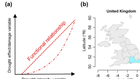
A common approach for assessing the negative conse-quences of natural hazards is the use of damage functions, variously called vulnerability functions or stage–damage curves depending on the damage variable used and on author conventions (e.g., Michel-Kerjan et al., 2013; Papathoma-Köhle et al., 2015; Tarbotton et al., 2015). Such damage functions are usually continuous curves relating the hazard intensity (e.g., inundation depth or wind velocity) to the neg-ative effects of the hazard, often expressed as a damage ratio of buildings. Transferring the concept of (empirical) dam-age functions to drought risk assessment presents many chal-lenges and has only recently begun to be addressed (Nau-mann et al., 2015). The main challenges can be conceptu-alized as follows: first, what is a suitable indicator charac-terizing the drought hazard (abscissa in Fig. 1a)? Drought is known as a multidimensional hazard affecting different do-mains of the hydrological cycle and with different response times (Wilhite and Glantz, 1985). Second, what is a suit-able damage varisuit-able for drought effect/damage (ordinate in Fig. 1a)? This is particularly challenging given that many negative consequences of drought, hereafter drought impacts, are non-structural and hard to quantify or monetize (e.g., lo-cal water supply shortages or restrictions on domestic water use, impaired navigability of streams, or ecological impacts such as irreversible deterioration of wetlands or fish kills) (Logar and van den Bergh, 2013). Also, there is a paucity of drought impact data with sufficient spatial and temporal resolution except for the agricultural sector (Bachmair et al., 2016b). The third challenge is identifying an adequate func-tional relationship for relating hazard intensity to a damage variable (red lines in Fig. 1a).

Regarding the first challenge (hazard intensity variable), several authors have empirically assessed which drought indicators are best linked to certain drought impact types such as, for example, vegetation stress and agricultural im-pacts, restrictions regarding water supply, or power gener-ation (e.g., Bachmair et al., 2016a; Blauhut et al., 2016; Lorenzo-Lacruz et al., 2013; Stagge et al., 2015b; Stahl et al., 2012; Vicente-Serrano et al., 2013). These drought in-dicators tend to be measures of hydrometeorological

vari-Figure 1. (a)Schematic examples of drought impact functions (red lines), and(b)location of the Southeast England study area (blue shading) among the NUTS1 regions of the UK.

ables which are relatively easy to quantify objectively, such as rainfall. Regarding the second challenge (drought damage variable), studies include a variety of data types representing the drought impact, including crop yield (e.g., Hlavinka et al., 2009; Naumann et al., 2015; Potopová et al., 2015; Quir-ing and Papakryiakou, 2003), wildfire occurrence (e.g., Gud-mundsson et al., 2014), drought-induced building damage (Corti et al., 2011), and hydropower production (Naumann et al., 2015). While the above data relate to one specific type of drought impact, text-based reports on drought impacts as assembled by the US Drought Impact Reporter (DIR) (Wil-hite et al., 2007) and the European Drought Impact report Inventory (EDII) (Stahl et al., 2016) provide information on different types, including indirect and non-market impacts (e.g., ecological impacts, impacts on human health). How-ever, for empirical damage functions such qualitative data need to be quantified, although this transformation inevitably introduces uncertainties. A few studies exploited text-based impact reports from the EDII by converting them into binary time series of impact occurrence (Blauhut et al., 2015b, 2016; Stagge et al., 2015b). Building on these efforts, Bachmair et al. (2015, 2016a) derived the number of impacts based on text-based data, providing a surrogate measure of impact severity. The suitability of these different impact quantifica-tion methods has not yet been systematically assessed.

The aim of this study is to develop empirical “drought im-pact functions” based on text-based reports from the EDII as surrogate information on drought damage and thereby as-sess possibilities and limitations of transferring the concept of damage functions to drought. Specifically, we test

– the effect of different methods of quantifying text-based drought impact information and

– the predictive performance of three data-driven models for linking drought intensity with drought impacts. We use a selection of standardized hydrometeorological indices as drought hazard indicators.

2 Data 2.1 Study area

We selected Southeast England (SEE) as a case study for developing the drought impact functions (Fig. 1b). This is a level 1 region of the Nomenclature of Units for Territo-rial Statistics (NUTS1), a spatial unit used in the European Union. The reasons for choosing SEE include the good data availability in the EDII for this region and the importance of drought risk assessment for this area given the severe droughts that have occurred in southeastern UK in the past (e.g., Kendon et al., 2013; Marsh, 2007). The southeast is one of the driest parts of the UK, but with some of the highest water demands. The region hosts a large population, approx-imately 9 million (Office for National Statistics, 2017), and high concentrations of commercial and industrial activity. Consequently, parts of the region are already water stressed, with pressures on the water environment expected to increase in future (Environment Agency, 2017). The EDII drought im-pacts for the SEE study area mainly consists of imim-pacts on the water supply and on freshwater ecosystems.

2.2 Predictors

As candidate predictors we selected the commonly used drought indicators Standardized Precipitation Index (SPI) (McKee et al., 1993) and Standardized Precipitation Evap-oration Index (SPEI) (Vicente-Serrano et al., 2010) of ac-cumulation periods of 1–6, 9, 12, and 24 months (hereafter SPI-n or SPEI-n). The SPI (SPEI) compares the total pre-cipitation (climatic water balance) of a certain location over a period of n months with its multiyear average (Vicente-Serrano et al., 2010; Zargar et al., 2011), so that negative val-ues of the SPI and SPEI indicate dryer than average tions and positive values indicate wetter than average condi-tions. SPI and SPEI are based on E-OBS gridded rainfall and temperature data (v12.0, 0.25◦spatial resolution) (Haylock et al., 2008). We used the R package “SCI” (Gudmundsson and Stagge, 2014) for SPI and SPEI calculation (gamma dis-tribution for SPI; generalized logistic disdis-tribution for SPEI;

standardization period for both variables: 1970–2012). Evap-otranspiration was determined using the Hargreaves–Samani method (Hargreaves and Samani, 1982). For each month we calculated the regional average of all E-OBS grid cells falling within the polygon covering SEE. The regional av-erage was chosen since Bachmair et al. (2015) found little difference between the performances of different regional in-dicator metrics. The SPI/SPEI accumulation durations reflect the water deficit accumulated in the SEE area over that dura-tion. As additional predictors, used to account for temporal trend and seasonality, we chose the year (Y) and the month (M, expressed as a sinusoid) of impact occurrence (Bach-mair et al., 2016a). For parts of the analysis the impact data of the preceding month were introduced as a further predictor to address autocorrelation of residuals (see Sect. 2.3 for how impact data were prepared). All predictor time series have monthly resolution. That is, although most of the SPI and SPEI accumulation periods are longer than a month, each in-dex is calculated for a moving window that is shifted one month at a time.

2.3 Drought impacts

Drought impact information for our SEE case study region comes from the EDII (Stahl et al., 2016), accessible at http: //www.geo.uio.no/edc/droughtdb/. The EDII contains text-based reports on drought impacts. Each report states (i) the location of occurrence (making reference to administrative regions at different NUTS levels), (ii) the time of occurrence (at least the start and end year), and (iii) the type of im-pact (assignment to predefined imim-pact categories and sub-types). For quantitative analysis these reports need to be con-verted into time series of impact information. We tested three different approaches of impact counting to address the un-certainty associated with impact report quantification. The general procedure follows previous studies (Bachmair et al., 2015, 2016a). For our analysis monthly time series are used. Not all impact reports state the start and end month of impact occurrence; if only information about the season was avail-able, we assumed drought impact occurrence during each month of this season (winter is DJF, spring is MAM, sum-mer is JJA, fall is SON). Impact reports only stating the year of occurrence, or with incomplete information about impact category or subtype, were omitted.

The impact counting methods are as follows:

1. Only presence versus absence of drought impacts per month is considered (Blauhut et al., 2015b, 2016; Stagge et al., 2015b), resulting in binary time series of impact occurrence (hereafterI).

2. All impact reports are counted. If an impact report states

“pub-lic water supply” seven impact subtypes may be speci-fied, ranging from local water supply shortage (e.g., dry-ing up of sprdry-ings/wells, reservoirs, streams) over bans on domestic and public water use (e.g., car washing, wa-tering the lawn/garden, irrigation of sport fields, filling of swimming pools) to increased costs/economic losses (Stahl et al., 2016). In total, there are 15 different impact categories in the EDII, each with its own set of subtypes. 3. An impact report assigned to one impact category only counts once, independent of how many impact subtypes are specified. The resulting time series shows the same dynamic as for method 2 but has lowerNI.

NI provides a measure of impact severity, but the

infor-mation is likely more uncertain than binary data. For our analysis we considered total impacts in SEE (all impact cat-egories) and two different subsets: water supply impacts and impacts related to freshwater ecosystems. These two impact categories make up the dominant part of the total impacts in SEE. As a consequence of the specific counting decision as well as the dynamic nature of the EDII, to which new entries may have been added and amendments or correction to ex-isting entries may have been made in the meantime, the time series used in this study may differ slightly from those used in previously published studies.

3 Methods

3.1 Data-driven models

To establish a functional relationship between drought indi-cators (and further predictors) and drought impactsI orNI,

we tested three different models:

1. logistic regression (LG) for the presence or absence of impact data as a binary response variable (Blauhut et al., 2015b, 2016; Stagge et al., 2015b);

2. zero-altered negative binomial regression; this paramet-ric model for count data is also known as a “hurdle” model (HM) (Zeileis et al., 2008); and

3. a “random forest” (RF) model (Breiman, 2001), which is an ensemble of regression trees.

Logistic regression was selected because it has been pre-viously used for drought impact modeling (Blauhut et al., 2015b; Gudmundsson et al., 2014). For modeling count data we aimed to explore the predictive performance of one para-metric model and a non-parapara-metric alternative. Since the im-pact data contain many zeros, we selected the HM, which is capable of dealing with excess zeros (Zeileis et al., 2008). The HM has been successfully applied to ecological datasets with zero inflation (Ver Hoef and Jansen, 2007; e.g., Potts and Elith, 2006). The RF model represents a flexible machine

learning approach that can handle non-linearities and pre-dictor interactions (Breiman, 2001; Liaw and Wiener, 2002). The RF model has been extensively used for many applica-tions in environmental science (e.g., Bachmair et al., 2016a; Catani et al., 2013; Oliveira et al., 2012; Park et al., 2016; Valero et al., 2016).

LG belongs to the class of generalized linear models (Zuur et al., 2009a). The (logit-transformed) probability of impact occurrence (π) is modeled as a linear function of the predic-torsxi following Eq. (1):

log _π

1−π

=α+X

i

βixi. (1)

The left-hand side represents the logit transformation; the model parametersαandβare estimated by maximum likeli-hood (McCullagh and Nelder, 1989).

The HM consists of two parts: a hurdle part for model-ing zero versus larger counts and a truncated count part for modeling positive counts (Zeileis et al., 2008). We selected a binomial model with logit link for the hurdle part (see LG); since the impact data are overdispersed (variance larger than theoretically expected, in this case larger than the mean) we selected a negative binomial model for the count part with log link. For details of this model see Zeileis et al. (2008) and Zuur et al. (2009b). We used the R package “pscl” for the implementation (Jackman, 2015).

The RF model is a machine learning algorithm where a large number of regression trees are grown on bootstrapped subsamples of the data (Breiman, 2001). We used the R pack-age “randomForest” (Liaw and Wiener, 2002). The default values were kept for all model parameters; the variablentree was set to 1000. Details about drought impact modeling us-ing RF can be found in Bachmair et al. (2016a). For this study, however, we found that results are best when applying a square root transformation to the response variable for the binary part of the time series and no transformation for the count part. We obtain the final modeled time series by run-ning the RF model twice with (a) square-root-transformed data and (b) untransformed data. The back-transformed out-put from model (a) is replaced with the outout-put from model (b) if the modeled number of impacts from (a) is≥1. Raw residuals refer to the difference between this final modeled time series and observed data.

3.2 Modeling approach

colinearity between the predictors, only the predictor show-ing the best correlation with the predictand (i.e., the impacts) was kept.

For RF there is no prior predictor selection; best perform-ing predictors are identified within the algorithm. Confidence intervals for LG and HM are computed using bootstrapping (resampling with replacement). For RF, confidence intervals are based on the predictions of all individual RF trees; each tree is constructed based on a bootstrapped subsample con-taining two-thirds of the data (Liaw and Wiener, 2002) .

For the analysis we used a censored time series based on years with drought impact occurrence rather than the entire time series (see Bachmair et al., 2015, 2016a). The rationale is that there may be a lack of impact reporting for certain drought events; hence we only focus on parts of the time se-ries with reported drought impacts. All months of all years with drought impact occurrence were selected plus an ad-ditional 6-month buffer before and after the drought year to include sufficient variability for model training. This resulted inn=234 months for total impacts,n=198 for water sup-ply impacts, andn=174 for freshwater ecosystem impacts.

To assess the model’s predictive performance we per-formed leave-one-out cross validation, i.e., each month is left out once for model training, and a prediction is made for this omitted month. We evaluated the model performance regarding its capability of predicting binary data and count data (HM and RF). For the binary performance evaluation we rounded the time series of LG; for HM and RF, data points < 1 were rounded, and data points > 1 were truncated to 1. We used the following performance metrics: hit rate (i.e., the proportion of predictions for which the presence or absence of impacts is correctly identified), false posi-tive, and false negative rate. The model performance met-ric for the count part of HM and RF is the Kling–Gupta ef-ficiency (KGE), which is based on the difference in mean, standard deviation, and correlation between the observed and the leave-one-out predicted series (Gupta et al., 2009). KGE lies between 1 (perfect fit) and negative infinity (worst fit).

4 Results

4.1 Selected predictors

The stepwise approach (see Sect. 3.2) resulted in the follow-ing predictors befollow-ing selected for the LG model: SPI-6, SPEI-24, andMfor modeling total impacts; SPI-6 and SPI-24 for water supply impacts; SPI-3, SPI-6, SPI-24, andY for fresh-water ecosystem impacts. The selected predictors for the HM are SPI-6 and SPEI-24 for the hurdle part and SPI-6 andY

for the count part (total impacts for both methods of impact quantification). For water supply and freshwater ecosystem impacts different predictors were automatically selected for both model parts and methods of impact quantification (water supply impacts: SPI of short, medium, and long

accumula-tion periods; freshwater ecosystem impacts: SPI and SPEI of short, medium, and long accumulation periods, andY). For RF, all predictor are used, yet similar predictors as for LG and HM were identified as most important during regression tree construction.

4.2 Fitted models

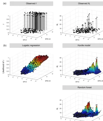
Figure 2 shows the dependence of the observed or modeled response variable (total impacts,NI quantified after method

3) on the selected predictors; note that only the dependence on SPI-6 and SPEI-24 is displayed although the models in-clude further predictors (e.g.,MandY). The top panels re-veal a complex relationship between drought indicators and observedI or NI. Impact counts occur not only for nega-tive drought indicator values: there are a few instances of

I for positive values of both drought indicators (front left quadrant), and several data points with impact counts yet negative indicator values for only one of SPI-6 or SPEI-24. The panels showing fitted data and an additional interpo-lated surface to aid visualization can be regarded as a three-dimensional version of the common two-three-dimensional dam-age functions based on one predictor. For LG, the fitted data reveal a comparably smooth increase of the likelihood of im-pact occurrence from positive to negative values for both se-lected drought indicators. For HM and RF, the response sur-face is more rugged. The RF model better captures observed

NI than HM, especially for cases with negative SPEI-24 but

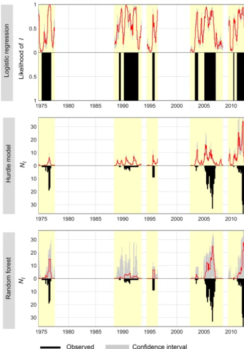
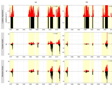
less negative SPI-6; HM strongly underestimates theseNI. Figure 3 additionally shows time series of observed versus fittedIorNIand confidence intervals. Both count data mod-els tend to underestimate medium to highNI. HM addition-ally shows estimates of impact occurrence when none oc-curred. The confidence intervals for LG and HM are rather narrow, whereas they are wider for RF. Note that for the im-pact quantification method 2 (same dynamics but higherNI),

the underestimation of highNI by RF is less pronounced,

whereas it is much more pronounced by HM (not shown). An analysis of the residuals revealed significant autocor-relation up to a lag of 8 months depending on the model and impact quantification method (see examples in Fig. 4). For RF, the autocorrelation of the residuals is less pronounced than for LG and HM. To take the autocorrelation into ac-count, impact information for the preceding month was in-cluded in the model. For the binary part of the model, this meant whether or not impacts occurred in the preceding month. For the count part, the number of impacts in the pre-ceding month was added as a predictor. The inclusion of this autoregressive part in the model generally resulted in a con-siderable decrease in the autocorrelation of the residuals. For HM, however, it also caused significant overprediction ofNI

Figure 2.Top row: dependence of the observed response variable (black dots) on SPI-6 and SPEI-24 (total impacts;NI: impact quantification

method 3). Bottom rows: fitted models (only SPI-6 and SPEI-24 are displayed although the models include further predictors).

4.3 Predictive performance

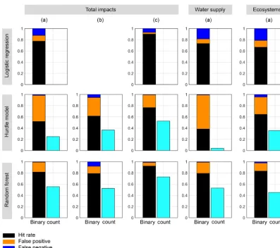
For each of the different models, the predicted series from the leave-one-out cross validation was compared with the ob-served series. The evaluation of the predictive performance considering binary data and count data (HM and RF) sepa-rately yielded the following findings (Fig. 5):

1. noticeable differences between models,

2. small differences between impact counting methods (i.e., all types of response data are equally well pre-dicted),

3. a positive effect of including impact information of the preceding month as an additional predictor, and

4. similar results regarding between-model differences for different impact subtypes.

Generally, for binary data, LG and RF perform similarly well with a hit rate of roughly 0.8; the hit rate of the hurdle model is distinctly lower (Fig. 5, columns 1–2). For count data, RF is superior to HM. The temporal dynamics ofNI

are better reproduced by RF than HM (see Fig. 6). However, underprediction of higher impact counts for the RF model lead to a lower mean and standard deviation than observed, resulting in KGE values less than 0.6. The HM shows an even stronger underprediction of highNI and frequent

count-Figure 3.Observed versus fitted time series ofI orNI (total

im-pacts;NI: impact quantification method 3).

ing method 3 (lowerNI)leads to a small but notable increase

in performance.

For all the models there is generally a positive effect of including the impact information from the preceding month as an extra predictor variable (Fig. 5, column 1 vs. 3). The hit rate of LG and RF increases to > 0.9, and KGE values in-crease by ca. 20 %. For HM, however, strong overestimation can be noticed for summer 2006 (Fig. 5). When subsetting the total impacts on water supply and freshwater ecosystems, respectively, the same general picture of between-model dif-ferences as for total impacts is seen. That is, RF and LG are similar regarding binary data, and RF is superior to HM for the count part (Fig. 5, columns 4–5). However, apart from this the results are varied. There is either a slightly in-creased or dein-creased predictive performance depending on the model, impact counting method, and binary versus count data performance metric (only impact counting method 2 is shown). Notable is a decreased performance of HM for wa-ter supply impacts, yet an increase for freshwawa-ter ecosystem impacts, compared with the prediction of total impacts.

Figure 4. Raw residuals for both count data models (total im-pacts;NI impact quantification method 3).(a)Models based on

selected predictors (see Sect. 3.2);(b)NI of preceding month as

additional predictor.

5 Discussion

im-Figure 5.Model performance metrics based on leave-one-out cross validation for total impacts and impacts on water supply and freshwater ecosystems.(a)NIafter impact quantification method 2;(b)NIafter impact quantification method 3;(c)as(a)but includingNIof preceding

month as additional predictor.

pact counts (only differentiating between impact categories but not subtypes) yielded better results. Overall, we recom-mend interpreting impact counts as a severity metric rather than as representing the true number of observed impacts. Since information about impact severity, in a quantitative (or at least systematically and objectively estimated) sense, is currently not available from the EDII database, exploring dif-ferent methods for counting the number of impact reports as we do here is in our opinion the best way currently to address impact severity.

Further sensitivity tests on the assumptions during im-pact quantification are desirable in future research, e.g., test-ing the effect of assigntest-ing a time of occurrence when im-pact reports only provide an approximate time indication. Testing three data-driven models revealed the superiority of RF with respect to predictive model performance. The dis-criminatory power of LG and the RF (based on square-root-transformed data) was comparable, with about 80 % of the binary data correctly predicted. However, in addition the RF model also provides information about impact severity. The

machine learning algorithm seems to be most capable of fit-ting “difficult” data points. For example, water supply re-lated impacts may persist because of low groundwater lev-els, despite shorter-term wet conditions. These cases mani-fest themselves as high observedNIfor very negative values of SPEI-24, but positive or only slightly negative values of SPI-6 (see Fig. 2). In fact, the selection of predictor variables for most of the models include a combination of such shorter-term and longer-shorter-term timescales of SPI or SPEI, sometimes together with the month (for seasonality) or year (for trend) of impact occurrence. While for the RF model all predictors are used, the above-named ones were identified as the most important ones.

Figure 6.Examples of observed versus modeled time series based on leave-one-out cross validation.(a)N_I after impact quantification method 2;(b)as(a)but includingNIof preceding month as additional predictor.

An increased performance of HM for more conservatively counted impact data (method 3) supports this speculation. One can infer that for text-based drought impact data non-parametric methods may be most suitable. Future work could test other machine learning or flexible approaches that have been applied to drought modeling (e.g., Morid et al., 2007). However, a slight improvement of HM performance by re-assessing the predictor selection may not be ruled out; we do not claim to have identified the optimal model by automatic predictor selection. Nevertheless, small tweaks regarding the in- or exclusion of certain predictors only yielded marginal differences. It can be noted that the study region is very di-verse geologically, which affects the response time of river flows to rainfall. The SPI duration showing the strongest re-lationship with monthly mean streamflow can vary greatly between catchments even over short distances due to the ge-ological heterogeneity of the southeast (Barker et al., 2016). For most catchments, Barker et al. (2016) found the cor-relation with streamflow to be strongest for SPI durations less than a year, but for very permeable catchments with a large groundwater contribution to flows, correlations re-mained strong up to the longest duration studied: 2 years. Hence, it seems reasonable to include SPI predictors repre-senting both the fast and the slow response to rainfall (the latter including groundwater as well as streamflow in perme-able catchments).

general as part of routine environmental and water resources monitoring. For example, on a more localized (catchment) scale it may be possible to develop impact functions using ecological response data (for example, in the case of SEE re-ported here), capitalizing on regular monitoring undertaken in the National Drought Surveillance Network (Dollar et al., 2013).

There are a range of potential applications for impact functions in water resources management, with two obvious examples being: long-term strategic drought and water re-sources planning and real-time monitoring and early warn-ing to support operational decision-makwarn-ing durwarn-ing drought events. For the case of long-term drought and water resources planning, in particular, scenarios provide a common tool to test and improve existing drought plans (for example, in re-lation to England as in this case study: Watts et al., 2012; Anderton et al., 2015). Currently such tests are mostly done at the level of individual water suppliers, with very specific failure functions, and generally such approaches focus on se-curity of water supply; Watts et al. (2012) argued that social or environmental impacts should be incorporated into such tests in future to enable the consequences of management de-cisions to be appreciated and thereby provide a more realistic test of Drought Plans. Similarly, impact functions may facili-tate more regional- to country-scale assessment of the risk of certain sectors to drought and hence enable the coordination of drought management plans across sectors. In a real-time context, an impact function enables the interpretation of a given drought index as a threshold or trigger of action. Im-pact functions thereby translate drought intensity expressed by a hydrometeorological indicator into the possibility of ex-periencing socioeconomic or ecological effects, based on his-torical experience. Currently, operational systems like the US Drought Monitor or the European Drought Observatory al-low the user to select different drought indices. We propose that in the future users should ideally also be able to select an index that provides information on whether socioeconomic or ecological effects can be expected for this drought in-tensity, which could be addressed by impact functions. This would go some way to countering a recognized deficiency in current monitoring and early warning systems, i.e., a capac-ity to quantify and eventually predict impacts on society and ecosystems (Bachmair et al., 2016b).

If near-real-time monitoring of drought impacts is avail-able, as is the case for the US DIR, impact predictions could be supported by impact information of the preceding time steps. Our analysis revealed an increase in predictive per-formance when including such knowledge. Furthermore, im-pact functions as surrogates for damage functions could be used with hazard scenarios to derive an estimate of risk (e.g., Stoelzle et al., 2014). However, drought impact functions represent a (rather loose) measure of severity; monetary risk estimates could only be derived by coupling them with ap-proaches to quantify the willingness to pay for the restora-tion of certain (ecosystem) services (Banerjee et al., 2013;

Logar and van den Bergh, 2013; Mens et al., 2015). Addi-tionally, hydro-economic models or engineering approaches could be tested against such empirically derived impact func-tions. A caveat is that our impact functions do not incorporate dynamics of vulnerability; i.e., the link between hydrometeo-rological indicators and impacts may change over time due to adaption and preparedness measures (Blauhut et al., 2015a), for example the increasing resilience of water supply sys-tems to drought. For monetary losses such changes may be accounted for (e.g., by price adjustment; Kron et al., 2012). In our case the variableY (year) may cater for trends in vul-nerability or impact reporting to some extent as suggested by Stagge et al. (2015b). Interestingly, the year is included as a predictor for all the models of freshwater ecosystem impacts, whereas the LG and HM use only SPI of different durations for estimating water supply impacts. However, clearly the in-clusion of a linear trend by year is necessarily an approxima-tion, and resilience changes episodically, with major events themselves being major catalysts for improvements in wa-ter governance or wawa-ter supply system resilience. To betwa-ter account for the dynamics of vulnerability, expert elicitation could be used to gain an understanding of the dynamics of adaption measures over time for a specific application and region. One would need to test whether quantifying such in-formation and adding it as further predictor variable would improve the reliability of impact functions.

In assessing the most suitable impact function for any ap-plication, further evaluation criteria may be useful in addi-tion to the predictive performance, such as the capability of extrapolation beyond the training data, interpretability and simplicity of communication, and ease of application. Es-pecially the ability of RF to predict impact occurrence for yet unexperienced drought scenarios needs to be explored Although the RF method means that complicated relation-ships between the (many) predictors and the predictand can be incorporated, the fewer predictors used in the LG and HM approaches make interpretation of the link between indica-tors and impacts more transparent. In the choice of modeling methodology, a balance therefore needs to be struck between these several different criteria.

6 Conclusion

in-formation for drought risk management. While the conver-sion of text-based reports into number of drought impact oc-currences is undeniably more uncertain than binary data of presence/absence of impact occurrence, it provides an ad-ditional measure of impact severity that was found reason-ably predictable. Unlike more commonly used damage func-tions linking one hazard variable to one particular type of damage, modeling the impacts of the multifaceted hazard of drought requires several drought indicators (in our case dif-ferent accumulation periods of SPI and SPEI). Out of the three models tested, the random forest model generally per-formed best. While logistic regression and the random forest model showed a similar discriminatory power for binary im-pact data, the random forest additionally predicts count data and thus information about impact severity. When using sub-sets of the total impacts (impacts on water supply and im-pacts on freshwater ecosystems) similar between-model dif-ferences are revealed. While the flexible machine learning algorithm seems most suitable for modeling the complex re-lation between drought indicators and text-based data, we do not claim to have generally identified the best model. Instead, our study showcases different methodological ap-proaches to developing drought impact functions based on text-based data, depending on data availability and purpose of analysis.

Data availability. The E-OBS gridded data on temperature and precipitation can be accessed at http://www.ecad.eu/download/ ensembles/download.php. E-OBS dataset were obtained from the EU-FP6 project ENSEMBLES (http://ensembles-eu.metoffice. com) and the data providers in the ECA&D project (http://www. ecad.eu). The content of the European Drought Impact Report In-ventory can be viewed at http://www.geo.uio.no/edc/droughtdb/.

Competing interests. The authors declare that they have no conflict of interest.

Special issue statement. This article is part of the special issue “Damage of natural hazards: assessment and mitigation”. It is a re-sult of the EGU General Assembly 2016, Vienna, Austria, 17–22 April 2016.

Acknowledgements. This study is an outcome of the Belmont Fo-rum project DrIVER (Drought Impacts: Vulnerability thresholds in monitoring and Early warning Research). Funding to the project DrIVER by the German Research Foundation DFG under the international Belmont Forum/G8HORC’s Freshwater Security programme (project no. STA-632/2-1) is gratefully acknowledged. Financial support for Cecilia Svensson and Jamie Hannaford within the DrIVER project was provided by the UK Natural Environment Research Council (grant NE/L010038/1). Financial support for Ilaria Prosdocimi while at CEH was provided by NERC/CEH National Capability funding.

Edited by: Thomas Thaler

Reviewed by: two anonymous referees

References

Anderton, S., Ledbetter, R., and Prudhomme, C.: Understanding the performance of water supply systems during mild to extreme droughts, Report SC120048/R, Bristol, Environment Agency, 61 pp., 2015.

Bachmair, S., Kohn, I., and Stahl, K.: Exploring the link between drought indicators and impacts, Nat. Hazards Earth Syst. Sci., 15, 1381–1397, https://doi.org/10.5194/nhess-15-1381-2015, 2015. Bachmair, S., Svensson, C., Hannaford, J., Barker, L. J., and Stahl,

K.: A quantitative analysis to objectively appraise drought indi-cators and model drought impacts, Hydrol. Earth Syst. Sci., 20, 2589–2609, https://doi.org/10.5194/hess-20-2589-2016, 2016a. Bachmair, S., Stahl, K., Collins, K., Hannaford, J., Acreman, M.,

Svoboda, M., Knutson, C., Smith, K. H., Wall, N., Fuchs, B., Crossman, N. D., and Overton, I. C.: Drought indica-tors revisited: the need for a wider consideration of environ-ment and society, Wiley Interdiscip, Rev. Water, 3, 516–536, https://doi.org/10.1002/wat2.1154, 2016b.

Banerjee, O., Bark, R., Connor, J., and Crossman, N. D.: An ecosystem services approach to estimating economic losses associated with drought, Ecol. Econ., 91, 19–27, https://doi.org/10.1016/j.ecolecon.2013.03.022, 2013.

Barker, L. J., Hannaford, J., Chiverton, A., and Svensson, C.: From meteorological to hydrological drought using standard-ised indicators, Hydrol. Earth Syst. Sci., 20, 2483–2505, https://doi.org/10.5194/hess-20-2483-2016, 2016.

Blauhut, V., Stahl, K., and Kohn, I.: The dynamics of vulnera-bility to drought from an impact perspective, in: Drought: Re-search and Science-Policy Interfacing – Proceedings of the Inter-national Conference on Drought: Research and Science-Policy Interfacing, CRC Press/Balkema, ISBN 9781138027794, 349– 354, 2015a.

Blauhut, V., Gudmundsson, L., and Stahl, K.: Towards pan-European drought risk maps: quantifying the link be-tween drought indices and reported drought impacts, En-viron. Res. Lett., 10, 14008, https://doi.org/10.1088/1748-9326/10/1/014008, 2015b.

Blauhut, V., Stahl, K., Stagge, J. H., Tallaksen, L. M., De Ste-fano, L., and Vogt, J.: Estimating drought risk across Eu-rope from reported drought impacts, drought indices, and vul-nerability factors, Hydrol. Earth Syst. Sci., 20, 2779–2800, https://doi.org/10.5194/hess-20-2779-2016, 2016.

Breiman, L.: Random Forests, Mach. Learn., 45, 5–32, https://doi.org/10.1023/A:1010933404324, 2001.

Briffa, K. R., Jones, P. D., and Hulme, M.: Summer moisture vari-ability across Europe, 1892–1991: An analysis based on the palmer drought severity index, Int. J. Climatol., 14, 475–506, https://doi.org/10.1002/joc.3370140502, 1994.

Corti, T., Wüest, M., Bresch, D., and Seneviratne, S. I.: Drought-induced building damages from simulations at re-gional scale, Nat. Hazards Earth Syst. Sci., 11, 3335–3342, https://doi.org/10.5194/nhess-11-3335-2011, 2011.

Dollar, E., Edwards, F., Laize, C., May, L., Acreman, M., and Wood, P.: Monitoring and assessment of environmental impacts of droughts (SC120024): work package 4, Final report, Bristol, UK, Environment Agency, (Report SC120024/R1, CEH Project no. C04647) (Unpublished), 47 pp., 2013.

Environment Agency: Water for people and the environment, Water resources strategy for England and Wales, Bristol, UK, available from: http://webarchive.nationalarchives.gov. uk/20140328091448/http://www.environment-agency.gov. uk/research/library/publications/40731.aspx, last access: 30 October 2017.

Gudmundsson, L. and Stagge, J.: SCI: Standardized Climate Indices such as SPI, SRI or SPEI, R package version 1.0-1, https://cran. r-project.org/web/packages/SCI/SCI.pdf (last access: 5 Novem-ber 2017), 2014.

Gudmundsson, L., Rego, F. C., Rocha, M., and Seneviratne, S. I.: Predicting above normal wildfire activity in southern Europe as a function of meteorological drought, Environ. Res. Lett., 9, 84008, https://doi.org/10.1088/1748-9326/9/8/084008, 2014. Gupta, H. V., Kling, H., Yilmaz, K. K., and Martinez, G. F.:

Decom-position of the mean squared error and NSE performance criteria: Implications for improving hydrological modelling, J. Hydrol., 377, 80–91, https://doi.org/10.1016/j.jhydrol.2009.08.003, 2009. Hargreaves, G. and Samani, Z.: Estimating potential

evapotranspi-ration, J. Irrig. Drain., 108, 225–230, 1982.

Haylock, M. R., Hofstra, N., Klein Tank, A. M. G., Klok, E. J., Jones, P. D., and New, M.: A European daily high-resolution gridded data set of surface temperature and pre-cipitation for 1950–2006, J. Geophys. Res., 113, D20119, https://doi.org/10.1029/2008JD010201, 2008.

Hlavinka, P., Trnka, M., Semerádová, D., Dubrovský, M., Žalud, Z., and Možný, M.: Effect of drought on yield variability of key crops in Czech Republic, Agr. Forest Meteorol., 149, 431–442, https://doi.org/10.1016/j.agrformet.2008.09.004, 2009.

Jackman, S.: pscl: Classes and Methods for R Developed in the Po-litical Science Computational Laboratory, Stanford University. Department of Political Science, Stanford University, Stanford, California, R package version 1.4.9, https://cran.r-project.org/ web/packages/pscl/pscl.pdf (last access: 29 November 2017), 2015.

Jongman, B., Kreibich, H., Apel, H., Barredo, J. I., Bates, P. D., Feyen, L., Gericke, A., Neal, J., Aerts, J. C. J. H., and Ward, P. J.: Comparative flood damage model assessment: towards a Eu-ropean approach, Nat. Hazards Earth Syst. Sci., 12, 3733–3752, https://doi.org/10.5194/nhess-12-3733-2012, 2012.

Kendon, M., Marsh, T., and Parry, S.: The 2010–2012 drought in England and Wales, Weather, 68, 88–95, 2013.

Kron, W., Steuer, M., Löw, P., and Wirtz, A.: How to deal properly with a natural catastrophe database – analysis of flood losses, Nat. Hazards Earth Syst. Sci., 12, 535–550, https://doi.org/10.5194/nhess-12-535-2012, 2012.

Liaw, A. and Wiener, M.: Classification and Re-gression by randomForest, R available from: ftp: //131.252.97.79/Transfer/Treg/WFRE_Articles/Liaw_02_

ClassificationandregressionbyrandomForest.pdf (last access: 13 January 2015), 2002.

Logar, I. and van den Bergh, J. C. J. M.: Methods to Assess Costs of Drought Damages and Policies for Drought Mitiga-tion and AdaptaMitiga-tion: Review and RecommendaMitiga-tions, Water Re-sour. Manag., 27, 1707–1720, https://doi.org/10.1007/s11269-012-0119-9, 2013.

Lorenzo-Lacruz, J., Vicente-Serrano, S. M., González-Hidalgo, J. C., López-Moreno, J. I., and Cortesi, N.: Hydrological drought response to meteorological drought in the Iberian Peninsula, Clim. Res., 58, 117–131, https://doi.org/10.3354/cr01177, 2013. Marsh, T.: The 2004–2006 drought in southern Britain, Weather, 62,

191–196, https://doi.org/10.1002/wea.99, 2007.

McCullagh, P. and Nelder, J. A.: Generalized Linear Models, Sec-ond Edn., Chapman & Hall/CRC Monographs on Statistics & Applied Probability, London, New York, 1989.

McKee, T. B., Doesken, N. J., and Kleist, J.: The relationship of drought frequency and duration to time scales, in Preprints, 8th Conference on Applied Climatology, Anaheim, California, 179– 184, 1993.

Mens, M. J. P., Gilroy, K., and Williams, D.: Developing system robustness analysis for drought risk management: an application on a water supply reservoir, Nat. Hazards Earth Syst. Sci., 15, 1933–1940, https://doi.org/10.5194/nhess-15-1933-2015, 2015. Merz, B., Kreibich, H., Schwarze, R., and Thieken, A.: Review

article “Assessment of economic flood damage”, Nat. Hazards Earth Syst. Sci., 10, 1697–1724, https://doi.org/10.5194/nhess-10-1697-2010, 2010.

Merz, B., Kreibich, H., and Lall, U.: Multi-variate flood damage as-sessment: a tree-based data-mining approach, Nat. Hazards Earth Syst. Sci., 13, 53–64, https://doi.org/10.5194/nhess-13-53-2013, 2013.

Michel-Kerjan, E., Hochrainer-Stigler, S., Kunreuther, H., Linnerooth-Bayer, J., Mechler, R., Muir-Wood, R., Ranger, N., Vaziri, P., and Young, M.: Catastrophe Risk Models for Evaluat-ing Disaster Risk Reduction Investments in DevelopEvaluat-ing Coun-tries, Risk Anal., 33, 984–999, https://doi.org/10.1111/j.1539-6924.2012.01928.x, 2013.

Morid, S., Smakhtin, V., and Bagherzadeh, K.: Drought forecasting using artificial neural networks and time se-ries of drought indices, Int. J. Climatol., 27, 2103–2111, https://doi.org/10.1002/joc.1498, 2007.

Naumann, G., Spinoni, J., Vogt, J. V., and Barbosa, P.: Assess-ment of drought damages and their uncertainties in Europe, Environ. Res. Lett., 10, 124013, https://doi.org/10.1088/1748-9326/10/12/124013, 2015.

Office of National Statistics: “GOR SYOA 1991-2015” sheet in Excel document “Regional Population Estimates for England and Wales 1971–2015.xls, available from: https://www.ons.gov.uk/peoplepopulationandcommunity/ populationandmigration/populationestimates/datasets/

populationestimatesforukenglandandwalesscotlandandnorthernireland, last access: 30 October 2017.

Papathoma-Köhle, M., Zischg, A., Fuchs, S., Glade, T., and Keiler, M.: Loss estimation for landslides in mountain ar-eas – An integrated toolbox for vulnerability assessment and damage documentation, Environ. Modell. Softw., 63, 156–169, https://doi.org/10.1016/j.envsoft.2014.10.003, 2015.

Park, S., Im, J., Jang, E., and Rhee, J.: Drought assess-ment and monitoring through blending of multi-sensor indices using machine learning approaches for differ-ent climate regions, Agr. Forest Meteorol., 216, 157–169, https://doi.org/10.1016/j.agrformet.2015.10.011, 2016.

Potopová, V., Štˇepánek, P., Možný, M., Türkott, L., and Soukup, J.: Performance of the standardised precipitation evapotranspi-ration index at various lags for agricultural drought risk assess-ment in the Czech Republic, Agr. Forest Meteorol., 202, 26–38, https://doi.org/10.1016/j.agrformet.2014.11.022, 2015.

Potts, J. M. and Elith, J.: Comparing species abun-dance models, Ecol. Model., 199, 153–163, https://doi.org/10.1016/j.ecolmodel.2006.05.025, 2006. Quiring, S. M. and Papakryiakou, T. N.: An evaluation of

agricul-tural drought indices for the Canadian prairies, Agr. Forest Me-teorol., 118, 49–62, 2003.

Schröter, K., Kreibich, H., Vogel, K., Riggelsen, C., Scherbaum, F., and Merz, B.: How useful are complex flood damage models?, Water Resour. Res., 50, 3378–3395, https://doi.org/10.1002/2013WR014396, 2014.

Schwarz, G.: Estimating the dimension of a model, Ann. Stat., 6, 461–464, 1978.

Smith, K. H., Svoboda, M., Hayes, M., Reges, H., Doesken, N., Lackstrom, K., Dow, K., and Brennan, A.: Local Observers Fill In the Details on Drought Impact Reporter Maps, B. Am. Me-teorol. Soc., 95, 1659–1662, https://doi.org/10.1175/1520-0477-95.11.1659, 2014.

Spekkers, M. H., Kok, M., Clemens, F. H. L. R., and ten Veldhuis, J. A. E.: Decision-tree analysis of factors influencing rainfall-related building structure and content damage, Nat. Hazards Earth Syst. Sci., 14, 2531–2547, https://doi.org/10.5194/nhess-14-2531-2014, 2014.

Stagge, J. H., Tallaksen, L. M., Gudmundsson, L., Van Loon, A. F., and Stahl, K.: Candidate Distributions for Climatological Drought Indices (SPI and SPEI), Int. J. Climatol., 35, 4027– 4040, https://doi.org/10.1002/joc.4267, 2015a.

Stagge, J. H., Kohn, I., Tallaksen, L. M., and Stahl, K.: Modeling drought impact occurrence based on meteorolog-ical drought indices in Europe, J. Hydrol., 530, 37–50, https://doi.org/10.1016/j.jhydrol.2015.09.039, 2015b.

Stahl, K., Blauhut, V., Kohn, I., Acácio, V., Assimacopoulos, D., Bi-fulco, C., De Stefano, L., Dias, S., Eilertz, D., Frielingsdorf, B., Hegdahl, T., Kampragou, E., Kourentzis, V., Melsen, L., Van La-nen, H., Van Loon, A., Massarutto, A., Musolino, D., De Paoli, L., Senn, L., Stagge, J., Tallaksen, L., and Urquijo, J.: A Euro-pean Drought Impact Report Inventory (EDII): Design and Test for Selected Recent Droughts in Europe, DROUGHT-R& SPI Technical Report No. 3, available from: http://www.eu-drought. org/technicalreports/3 (last access: 29 October 2017), 2012. Stahl, K., Kohn, I., Blauhut, V., Urquijo, J., De Stefano, L., Acácio,

V., Dias, S., Stagge, J. H., Tallaksen, L. M., Kampragou, E., Van Loon, A. F., Barker, L. J., Melsen, L. A., Bifulco, C., Musolino, D., de Carli, A., Massarutto, A., Assimacopoulos, D., and Van Lanen, H. A. J.: Impacts of European drought events: insights

from an international database of text-based reports, Nat. Haz-ards Earth Syst. Sci., 16, 801–819, https://doi.org/10.5194/nhess-16-801-2016, 2016.

Stoelzle, M., Stahl, K., Morhard, A., and Weiler, M.: Stream-flow sensitivity to drought scenarios in catchments with different geology, Geophys. Res. Lett., 41, 6174–6183, https://doi.org/10.1002/2014GL061344, 2014.

Tarbotton, C., Dall’Osso, F., Dominey-Howes, D., and Goff, J.: The use of empirical vulnerability functions to assess the re-sponse of buildings to tsunami impact: Comparative review and summary of best practice, Earth-Sci. Rev., 142, 120–134, https://doi.org/10.1016/j.earscirev.2015.01.002, 2015.

Thieken, A. H., Müller, M., Kreibich, H., and Merz, B.: Flood damage and influencing factors: New insights from the Au-gust 2002 flood in Germany, Water Resour. Res., 41, 1–16, https://doi.org/10.1029/2005WR004177, 2005.

UNISDR: Terminology on Disaster Risk Reduction, United Nations secretariat of the International Strategy for Disaster Reduction (UNISDR), Geneva, 2009.

Valero, S., Morin, D., Inglada, J., Sepulcre, G., Arias, M., Hagolle, O., Dedieu, G., Bontemps, S., Defourny, P., and Koetz, B.: Pro-duction of a Dynamic Cropland Mask by Processing Remote Sensing Image Series at High Temporal and Spatial Resolutions, Remote Sens., 8, 55, https://doi.org/10.3390/rs8010055, 2016. Ver Hoef, J. M. and Jansen, J. K.: Space–time zero-inflated

count models of Harbor seals, Environmetrics, 18, 697–712, https://doi.org/10.1002/env.873, 2007.

Vicente-Serrano, S. M., Beguería, S., and López-Moreno, J. I.: A multiscalar drought index sensitive to global warming: the stan-dardized precipitation evapotranspiration index, J. Climate, 23, 1696–1718, 2010.

Vicente-Serrano, S. M., Gouveia, C., Camarero, J. J., Beguería, S., Trigo, R., López-Moreno, J. I., Azorín-Molina, C., Pasho, E., Lorenzo-Lacruz, J., and Revuelto, J.: Response of vegetation to drought time-scales across global land biomes, P. Natl. Acad. Sci. USA, 110, 52–57, 2013.

Watts, G., von Christierson, B., Hannaford, J., and Lonsdale, K.: Testing the resilience of water supply systems to long droughts, J. Hydrol., 414, 255–267, 2012.

Wilhite, D. and Glantz, M.: Understanding: the drought phe-nomenon: the role of definitions, Water Int., 10, 111–120, https://doi.org/10.1080/02508068508686328, 1985.

Wilhite, D., Hayes, M., Knutson, C., and Smith, K.: Planning for drought: Moving from crisis to risk management, J. Am. Water Resour. As., 36, 697–710, https://doi.org/10.1111/j.1752-1688.2000.tb04299.x, 2000.

Wilhite, D. A., Svoboda, M. D., and Hayes, M. J.: Understanding the complex impacts of drought: A key to enhancing drought mit-igation and preparedness, Water Resour. Manag., 21, 763–774, https://doi.org/10.1007/s11269-006-9076-5, 2007.

Zargar, A., Sadiq, R., Naser, B., and Khan, F. I.: A re-view of drought indices, Environ. Rev., 19, 333–349, https://doi.org/10.1139/A11-013, 2011.

Zeileis, A., Kleiber, C., and Jackman, S.: Regression Mod-els for Count Data in R, J. Stat. Softw., 27, 1–25, https://doi.org/10.18637/jss.v027.i08, 2008.