Development of high-resolution multi-scale modelling system for
simulation of coastal-fluvial urban flooding
Joanne Comer, Agnieszka Indiana Olbert, Stephen Nash, and Michael Hartnett
Civil Engineering, College of Engineering and Informatics, Ryan Institute, National University of Ireland, Galway, University Road, Galway, Ireland
Correspondence to:Agnieszka Indiana Olbert ([email protected]) Received: 5 July 2016 – Discussion started: 18 July 2016
Revised: 16 December 2016 – Accepted: 5 January 2017 – Published: 16 February 2017
Abstract.Urban developments in coastal zones are often ex-posed to natural hazards such as flooding. In this research, a state-of-the-art, multi-scale nested flood (MSN_Flood) model is applied to simulate complex coastal-fluvial urban flooding due to combined effects of tides, surges and river discharges. Cork city on Ireland’s southwest coast is a study case. The flood modelling system comprises a cascade of four dynamically linked models that resolve the hydrody-namics of Cork Harbour and/or its sub-region at four scales: 90, 30, 6 and 2 m.
Results demonstrate that the internalization of the nested boundary through the use of ghost cells combined with a tai-lored adaptive interpolation technique creates a highly dy-namic moving boundary that permits flooding and drying of the nested boundary. This novel feature of MSN_Flood pro-vides a high degree of choice regarding the location of the boundaries to the nested domain and therefore flexibility in model application. The nested MSN_Flood model through dynamic downscaling facilitates significant improvements in accuracy of model output without incurring the computa-tional expense of high spatial resolution over the entire model domain. The urban flood model provides full characteristics of water levels and flow regimes necessary for flood hazard identification and flood risk assessment.
1 Introduction
Low-lying developments in coastal zones are exposed to nat-ural hazards such as storm surges, waves, tsunamis and/or high river flows which can lead to significant flooding. Coastal flooding can result in substantial economic and
so-cial impacts including loss of life, damage to property and disruption of essential services (Brown et al., 2007).
Coastal flooding results from a rise of sea water level above normal predicted tide level. On the European conti-nental shelf, coastal flooding is associated with storms gen-erated in the Atlantic Ocean that travel through, or in proxim-ity to, the shelf. Storm surges are important consequences of these storms – a temporary water setup resulting from synop-tic variation of atmospheric pressure and strong winds blow-ing towards the shelf, causblow-ing water to pile up against the coast. Surge physics is well understood in principle (Ponte, 1994); the mechanism of its propagation on the European continental shelf as a response to meteorological conditions (wind stress and atmospheric pressure signal separate) has been explained by Olbert and Hartnett (2010).
and Wicherson, 1999) providing high-resolution digital sur-face maps that can be used as model bathymetry (Marks and Bates, 2000). Although there are still problems with mapping urban areas and considerable post-processing is necessary to extract digital terrain model from digital surface models (Ma-son at al., 2007), the hydraulic/hydrodynamic models devel-oped using lidar data allow them to numerically propagate surge and tidal waves into coastal areas. Model accuracy and computational cost are still issues to be addressed.
The most common and simple approach to the modelling of coastal flooding in urban areas is to link (externally or dynamically) longitudinal 1-D or latterly averaged 2-D hy-draulic models with coastal models (e.g. Formaggia, 2001; Chen, 2007; Brown et al., 2007). Such a setup has two sig-nificant drawbacks. Firstly, 1-D/2-D hydraulic models work with the assumption that the lateral variations in velocity magnitudes are small, while in reality many coastal flood-plains (e.g. urban areas) contain channels that have a signif-icant influence on the development of inundation by provid-ing routes along which storm surges propagate inland (Bates et al., 2005) and therefore may lead to misrepresentation of localized flooding (Cook and Merwade, 2009; Mark et al., 2004). Secondly, numerical errors may be introduced when linking different models with different dimensions resulting from poor conservation of momentum (Yang et al., 2012). There is evidence of proven difficulty in ensuring that each model interprets the model inputs and boundary conditions in the same way (Hunter et al., 2008; Pender and Neelz, 2010). These problems may be overcome by application of a sin-gle hydrodynamic model to both coastal waters and coastal floodplains. Although such a model would allow smooth transition of the model solution between coastal waters and floodplains, the full solution at scales appropriate for flood inundation would incur a significant computational cost. On one hand, such models need to extend far enough offshore to capture the development and propagation of surge and to resolve the non-linear shallow-water dynamics (interactions between tides, surges and waves) at a resolution that is com-mensurate with flow features. On the other hand the model needs to include upstream river channels, tidal flats, low-lying land and urban areas which are susceptible to flood-ing at very fine resolution. This often results in a model setup that requires a large computational domain of which the area of particular interest (such as floodplains here) com-prises only a small percentage. For structured grid models such requirements are often cost-prohibitive, and the alterna-tive is to use lower resolution at the expense of accuracy. This means that model discretization is performed at scales well below those achievable with lidar data (the level of individual buildings in the case of urban flooding), meaning the highly resolved lidar data are not being optimally used (McMillian and Brasington, 2007). Some quite successful attempts have been made using unstructured-grid models allowing selective grid refinement (e.g. Yang et al., 2012; Robins et al., 2011); however, the computational demand of these models is high.
A relatively new approach to address this problem in high-resolution flood modelling makes use of continuing advances in computational resources through numerical domain de-composition and multi-core architecture runs (Sanders et al., 2010). This method, however, requires substantial computa-tional resources not commonly available yet.
In reality the modelling of coastal flooding (particularly in an urban environment) is a multi-scale problem that requires accurate solution at various scales ranging from coastal sea or estuary scale down to a dense street network of the inun-dated urban area. In the case of single rectilinear grid mod-els, which are still the most commonly used hydrodynamic models, this spatial-resolution problem may be overcome by grid nesting; this involves embedding higher-resolution grids within a lower-resolution global large-scale grid model. Such a solution allows users to specify high resolution in a sub-region of the model domain without incurring the compu-tational expense of fine resolution over the entire domain. Nonetheless, the nested model for simulation of floodplains must be very carefully chosen due to the flooding and drying properties of such zones; most nested models developed to date do not incorporate flooding and drying as they have been developed specifically for large-scale application where this phenomenon is not important (e.g. ROMS; Haidvogel et al., 2008) or, even if they incorporate flooding and drying such as Mike21 (DHI Software, 2001), flooding and drying of open boundaries are prohibited. This problem has been recently re-solved in the multi-scale nested flood (MSN_Flood) model of Nash and Hartnett (2010), which allows flooding and drying both within the domain and along boundaries, while main-taining accuracy and computational efficiency. This model is ideally suited for high-resolution modelling of urban flood-ing and, therefore, has been adopted for further development in this research.
In this context, the authors present in this paper for the first time the application of the state-of-the-art flood model MSN_Flood to complex coastal-fluvial urban flooding in estuary-lying Cork city, which is subject to the combined ef-fects of tides, surges and river discharges. The primary ob-jectives of this paper then are to present the development of this model and to critically examine its capability to fore-cast/hindcast the urban inundation. It will be demonstrated in this paper that through the novel solution to the nested boundary, the so-called moving boundary, the nested model allows simulation of the propagation of open-sea conditions up to the tidally active river upstream as well as rural and ur-ban floodplains in a computationally efficient manner with-out compromising model accuracy or stability.
lar, wetting and drying routine, computational efficiency, and accuracy of simulated water elevations and velocity fields are subject to in-depth analysis in this research.
This paper is organized as follows: Sect. 1 describes the motivation for this research and related work; Sect. 2 de-scribes modelling, model setup and datasets; Sect. 3 presents and compares numerical model results with observed datasets; Sect. 4 discusses the advantages the MSN_Flood modelling system; and finally Sect. 5 contains conclusions from the research.
2 Methodology
In this section a modelling system for coastal flood inunda-tion is described along with the datasets and model setup for the Cork city flood event.
2.1 Modelling framework
Many flood inundation events in urban environments have been modelled using simple hydraulic models, such as HEC-RAS (Pappenberger et al., 2005) or LISFLOOD-FP (Bates and De Roo, 2000), incapable of simulating flood water ve-locities required for accurate determination of flood wave propagation routes and assessment of risks associated with a certain flood flow magnitude. A more realistic analysis can be achieved using a hydrodynamic model that resolves both the continuity and momentum equations throughout the en-tire domain.
Here, the MSN_Flood model was applied to Cork city us-ing a cascade of four nested grids to describe hydrodynam-ics at various scales with particular interest in water eleva-tions and velocity fields over the inundated area. This nested model facilitates the refinement of spatial resolution in Cork Harbour from 90 m at the outer reaches of the harbour down to 2 m in the streets of Cork city.
2.2 Hydrodynamics
MSN_Flood is a two-dimensional, depth-averaged, finite-difference model, and its solver is based on the alternate di-rection implicit (ADI) solver developed by Falconer (1984) (Lin and Falconer, 1997; Nash and Hartnett, 2010). The governing differential equations used in the model to deter-mine the water elevation and depth-integrated velocity fields in the horizontal plane are based on integrating the three-dimensional continuity and Navier–Stokes equations over the water column depth. Assuming vertical accelerations are negligible compared with gravity and that the Reynolds stresses in the vertical plane can be represented by a Boussi-nesq approximation, then the depth-integrated continuity and
∂t ∂x ∂y
momentum equation inxdirection,
∂qx
∂t +β
∂U q
x
∂x +
∂U qy
∂y
=f qy−gH
∂ζ ∂x
+ρaC ∗W
x(Wx2+Wy2)1/2
ρ −
gU (U2+V2)1/2 C2
+2 ∂
∂x εH∂U ∂x + ∂ ∂y εH ∂U ∂y + ∂V ∂x , (2)
wheret is time;U andV are depth-averaged velocity com-ponents in thex and y directions, respectively; qx and qy
are depth-integrated volumetric flux components in thexand
ydirections (qx=U H;qy=V H);His total water depth;β
is a momentum correction factor for non-uniform vertical ve-locity profile;f is a Coriolis parameter (=2ωSinφ, where
ωis the angular velocity of the earth’s rotation andφis ge-ographical latitude);gis gravitational acceleration;ρaandr
are air and fluid densities, respectively;C∗is an air–water in-terfacial resistance coefficient;WxandWyare wind velocity
components inxandydirections, respectively;Cis a Chezy bed roughness coefficient; andεis depth mean eddy viscos-ity.
2.3 Nesting structure and procedure
MSN_Flood consists of one outer coarse grid, called the par-ent grid (PG), into which one or more inner fine grids (child grids, CGs) are one-way nested. The model also enables mul-tiple nesting such that a child grid may also be a parent to an-other child. In this way, multi-scale nesting can be specified enabling high spatial resolution in areas of interest. PG and CG models are dynamically coupled and synchronous. An overview of the nesting procedure is schematically presented in Fig. 1. As can be seen, the time integration is a bottom-up approach where PG can be advanced in time only when all of its children are integrated to the parent current time. The ADI solution technique to solve the governing continuity and momentum equations requires the sub-division of each time step into two half-time-steps. The nesting procedure, for each nesting level, is summarized in the following 5 steps:
1. integrate outermost parent grid one time step (t+1tp);
2. extract parent grid data and interpolate (spatially and temporally) along child grid boundary to next time lev-els of child grid (t+1/21tc)and (t+1tc);
3. integrate child grid 1 time step (t+1tc);
Figure 1.The nesting procedure for a single level of nesting and one variable only – water surface elevation,ζ.
5. return to step 1 and continue.
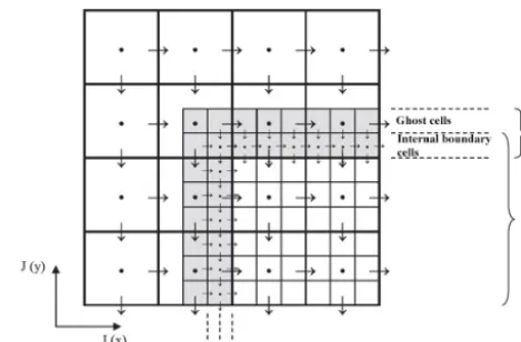
The nesting procedure is similar in principle to other nested models (Holt et al., 2009; Korres and Lascaratos, 2003; Nittis et al., 2006), but the uniqueness of MSN_Flood is a novel approach to boundary formulation through an in-corporation of ghost cells (GCs) in a manner that the nested boundary operates as an internal boundary. GCs are speci-fied adjacent to nested boundaries so that the boundary con-figuration consist of two rows/columns of CG cells: inter-nal boundary cells and the adjacent exterior ghost cells. A schematic of the general configuration of the nested bound-ary is shown in Fig. 2. In this internal boundbound-ary approach, PG boundary data are specified to both the ghost cells outside the CG domain and to the internal boundary cells, allowing the governing equations of motion at the internal boundary grid cells to be formulated and solved in the same way as inte-rior grid cells. This enables accurate specification and con-servation of incoming fluxes of mass and momentum along the boundaries of the nests. To demonstrate benefits of this approach, the finite-difference formulation for the advective term in the momentum equation, which is key to momentum conservation, at boundary cells becomes
∂U qx ∂x =
[U (x+1x, y)+U (x, y)]
2 .
[qx(x+1x, y)+qx(x, y)]
2
−[U (x, y)+U (x−1x, y)]
2 .
[qx(x, y)+qx(x−1x, y)]
2
. (3)
For comparison, in a boundary formulation without ghost cells, the derivative∂U qx/∂xwould be set to 0 as ghost cell
grid pointsU (x+1x, y)orU (x−1x, y)would not exist; therefore momentum would not be conserved between parent grid and child grid.
An important feature of the nesting approach in MSN_Flood is the implementation of moving boundaries along the boundary of the nested domains. The flooding and drying routine originally developed by Falconer and Chen (1991) is implemented in MSN_Flood; this boundary formulation allows the model to be applied to areas of inter-tidal zone or coastal flooding where there is typically a
con-Figure 2.Schematic illustration of the internal boundary configura-tion for 3 : 1 nesting ratio.
siderable degree of alternate flooding and drying throughout the domain. The flooding and drying routine by Falconer and Chen has been extensively tested in laboratory conditions and natural waterbodies and shown to be stable and robust. How-ever, when the nested boundary was subject to flooding and drying, despite the overall improvement in mass and momen-tum conservation along the nested boundary, significant er-rors were found to occur near the boundary in areas of flood-ing and dryflood-ing. This problem was overcome by implemen-tation of an adaptive interpolation scheme which uses linear interpolation or zeroth-order interpolation depending on the status (wet or dry) and the configuration of parent grids along the boundary interface. More details of the method can be found in Nash (2010). This adaptive interpolation in com-bination with ghost cell and internal boundary formulation ensures the stable flooding and drying of boundary cells.
con-Figure 3.Bathymetry of Cork Harbour (m) with selected locations. Red dot denotes location of Cork Harbour on the coast of Ireland.
ditions were tested, namely Dirichlet condition, flow relax-ation condition and radirelax-ation condition. Extensive numeri-cal testing showed that the most stable and accurate model solution could be achieved by implementing the Dirichlet boundary condition. Accuracies of various interpolation and boundary condition schemes were analysed and compared in Nash and Hartnett (2014).
Reduction in boundary errors due to the accurate develop-ment of boundary operators and more accurate mathematical formulation of the nested boundary yielded significant im-provements in conservation of mass and momentum between parent and child grids. This in turn improved model stabil-ity at the nested boundary and CG accuracy. These features make MSN_Flood highly applicable to modelling complex coastal flooding events as in the current test case, where the nested boundary is located in the flooding and drying zone, and therefore its length changes dynamically throughout the flooding event. This non-continuous moving boundary fea-ture is the subject of in-depth investigation in this research. 2.4 Study area description and model setup
Cork Harbour, in the southwest of Ireland, is a shallow (aver-age depth 8.4 m) meso-tidal estuary with typical spring tide ranges of 4.2 m. Return levels of tides for 2- and 100-year return periods are 4.45 and 4.52 m above chart datum, re-spectively, while surge residual return levels for the same return periods are 0.56 and 0.85 m, respectively (Olbert et al., 2013). The Cork Harbour domain is presented in Fig. 3. Cork city is a densely populated urban area of approximately 120 000 people, located at the mouth of the River Lee, which drains into Cork Harbour. Tidal components of flooding in Cork city are due to combinations of high astronomical tides
Figure 4.Four-level nesting structure of Cork Harbour and Cork city nested models.
and storm surges generated in the open ocean and propagat-ing into the harbour and throughout the city streets. The River Lee corridor flows from west to east along the post-glacial valley into the Lee proper, through Cork city, into Lough Ma-hon and Cork Harbour, and south into the Atlantic Ocean. In the city, the River Lee bifurcates into the north and south channels around the Mardyke area and merges again at the eastern edge of the city. The river flows for 2- and 100-year return periods are 208.6 and 307.7 m3s−1, respectively (Hal-crow, 2008). Sea water intrusion up the river is bounded by a weir located 8 km upstream from the river mouth.
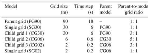
MSN_Flood was used in this research to develop a coastal-urban hydraulic model capable of simulating fluvial and coastal flooding in Cork city. The model grid needs to be set up to include not only river channel and urban floodplains but also offshore waters necessary to resolve the non-linear hy-drodynamics. The Cork Harbour/city model is therefore con-figured as a four-level cascade of dynamically linked nested grids that resolve the hydrodynamics of the region at spa-tial scales of 90, 30, 6 and 2 m. Each coarser grid provides boundary conditions to the next-finer grid; i.e. the 90 m grid provides boundary conditions to the 30 m grid, the 30 m grid provides boundary conditions to the 6 m grid etc. Figure 4a illustrates the extent of each grid and the nesting structure, while Fig. 4b shows details of the high-resolution 6m grid and the 2 m urban flood grid.
Table 1.Configuration of nested models.
Model Grid size Time step Parent Parent-to-model (m) (s) model grid ratio
Parent grid (PG90) 90 18 – 1 : 1 Single grid (SG30) 30 6 PG90 1 : 1 Child grid 1 (CG30) 30 6 PG90 3 : 1 Child grid 2 (CG06) 6 0.6 CG30 5 : 1 Child grid 3 (CG02) 2 0.2 CG06 3 : 1 Single grid (SG02) 2 0.2 CG06 1 : 1
child grid (CG02) is entirely embedded within CG06 and is used to simulate urban flooding of Cork city. The nesting ra-tios of 3 : 1 and 5 : 1 used in this setup are in line with nesting ratios used in other studies (e.g. Spall and Holland, 1991). Configurations of the nested models are summarized in Ta-ble 1.
Open-boundary conditions to the MSN_Flood parent grid, PG90, are provided as total water elevations containing tidal and surge signals extracted from an ocean model of the east-ern North Atlantic (Olbert and Hartnett, 2010). The surface boundary of the MSN_Flood model is forced by 10 m wind fields and mean sea level atmospheric pressure obtained from the regional analysis ERA-40 model (Uppala et al., 2005) and operational model first-guess dataset (Simmons et al., 1989). River Lee discharges from gauge station 19011 were provided by the Office of Public Works (OPW), Ireland. Admiralty chart data were used to develop the bathymetric model of Cork Harbour, while high-resolution lidar data pro-vided by the OPW were used to construct the high-resolution urban digital bathymetric model. The channel of the River Lee was included in the model based on cross-sectional sur-vey data also provided by the OPW from an extensive sursur-vey of the River Lee catchment in 2008.
2.5 Verification
The numerical model skill was assessed by statistically com-paring observations and model solutions. Following statisti-cal measures were used:
– root mean square error,
RMSE= " 1 N N X
n=1
(Yn−Xn)2
#1/2
; (4)
– root mean square difference between model and observa-tions, RMSdiff= " 1 N N X
n=1 (Yn)2
#1/2 − " 1 N N X
n=1 (Xn)2
#1/2
; (5)
– centred root mean square difference,
RMSD= " 1 N N X
n=1
Yn−Y− Xn−X
2
#1/2
, (6)
whereX andY are the mean values of variablesX andY, respectively, forN observations. These measures were also used to inter-compare time series of models of different res-olutions.
The spatially comparative measures between various mod-els are based on spatial distribution of errors between fine-and coarse-resolution models fine-and are quantified using the following expressions:
– tidally averaged relative errors,
RET=
N
P
n=1
|Yn−Xn| N
P
n=1
|Xn|
·100; (7)
– domain-averaged relative error, RED=
RET
M ; (8)
– absolute error,
AET=
N
P
n=1
|Yn−Xn|
N ; (9)
– relative difference, RD=|Xn−Yn|
Xn
, (10)
whereXandY are higher- and coarser-resolution solutions, respectively;nis the output time over a tidal cycle;N=25 is the total number of tidal cycles; andMis the number of discrete points in space.
3 Results
Figure 5.Comparison of computed and measured velocities at point P1in Passage West. Point location shown in Fig. 3.
3.1 Validation of the nesting procedure 3.1.1 PG90 model
Firstly, the performance of the low-resolution 90 m parent grid (PG90) model was assessed. Figure 5 compares current velocities simulated by the PG90 model with measured data at Passage West in Cork Harbour over a spring tidal cycle (see Fig. 3 for point P1 location). Results show that, although patterns of currents through flood and ebb conditions are rel-atively well predicted, the slack water conditions, where ve-locities are generally smaller, are not reproduced correctly by the PG90 model. A higher-resolution single-grid (SG30) model at 30 m grid spacing was developed to test the accu-racy of PG90. The same domain extents (Fig. 4) and the same physical conditions were specified to the SG30 and PG90 models. As shown in Fig. 5, an increased resolution of the model significantly improves model predictions throughout the tidal cycle and particularly during periods of slack water. The spatial distribution of PG model error was quanti-fied by calculating the tidally averaged relative errors RET,
expressing a percentage error in a PG solution relative to a higher-resolution SG reference solution (Eq. 7). Figure 6 shows the distribution of RETin PG velocities in Cork
Har-bour; it can be seen that the errors generated by the PG model are well over 30 % at certain locations within the harbour (harbour entrance, along the coastline, narrow channels and estuaries), so increasing the resolution from 90 to 30 m leads to significant reduction in the error. However, improvements in accuracy due to higher spatial resolution come at a high computational cost, which for the SG model (80 min for 50 h run) is 9 times that of the PG model (9 min for 50 h run). The use of a nested model is then a justifiable and favourable solution.
In the course of extensive validation, the time series of PG90 and SG30 were also inter-compared. Figure 7 shows water elevations and current velocities in Lough Mahon (see Fig. 3 for point C1 location). Water elevations computed by both models are in very good agreement. In contrast,
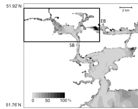
cur-Figure 6.Current velocity RET (%) in PG90 relative to SG30.
Black box shows the extent of CG30 and locations of nested bound-aries. EB – east boundary; SB – south boundary.
Figure 7.Comparison of(a)water elevations and(b)current veloc-ities at point C1 in Lough Mahon. Point location shown in Fig. 3.
rent velocities are significantly overpredicted by the PG90 model. Linear regression of current speeds of PG90 against SG30 solution is shown in Fig. 8. As can be seen from this figure, the correlation coefficient between PG90 and SG30 is 0.89, while slope and intercept arem=1.24 andc=0.03, respectively.
3.1.2 CG30 model
Figure 8.Comparison of modelled velocities for various grid setups at point C1 in Lough Mahon (point location shown in Fig. 3). Time series data are overlain by a linear trend.
The first level child grid, CG30, was located in the north-west part of Cork Harbour, with the centrally located Lough Mahon (directly feeding to the River Lee estuary) being the area of interest. The boundaries for the CG30 domain were chosen based on the RETdistribution plot for the PG90
cur-rent velocities presented in Fig. 6. The upper section of Pas-sage West, connecting Lough Mahon with Cork Lower Har-bour, was selected as a suitable southern boundary (SB) due to its relatively low RET, while the closest suitable location
for the eastern boundary (EB) was at a much greater distance from Lough Mahon due to generally high PG inaccuracies in the North Channel.
The accuracy of the CG30 boundary location was assessed by comparing the net fluxes of mass and momentum across the corresponding interfaces in the PG90, SG30 and CG30 models. Net fluxes were calculated normal to boundaries. Mass and momentum fluxes through the SB and EB bound-aries are compared in Figs. 9 and 10, respectively. It can be seen that the predominant forcing boundary for the CG30 do-main is the SB boundary. The tidally averaged errors in PG90 fluxes relative to the SG30 were approximately 4 % for both mass and momentum, indicating a high level of PG90 accu-racy. At the EB boundary, the PG90 accuracy was slightly lower, resulting in error in PG90 mass flux of 5 % and mo-mentum flux of 10 %. However, this boundary accounted for a smaller portion of the total boundary forcing, and its dis-tant location from the area of interest allowed boundary er-rors more time to dissipate. The tidally averaged erer-rors in CG30 fluxes (both mass and momentum) relative to PG90 fluxes were less that 2 % at both boundaries, demonstrating high levels of conservation from parent grid to child grid.
Relative error analysis was also carried out for the entire CG30 model domain with respect to water elevations and ve-locities, and results of these analyses are summarized in Ta-ble 2. The domain-averaged relative error (Eq. 8) in the PG90 water elevations relative to the SG30 were 5.9 %, while in the CG30 model this error was reduced to 1.1 %. The extent of
Figure 9.Comparison of(a)mass and(b)momentum fluxes across EB boundary; PG90 and CG30 time series are coincident.
Table 2.Summary of error analyses for PG90 and CG30 models within CG30 model area.
SG30
Error analyses parameter PG90 CG30
Water elevation:
– RED[%] 5.9 1.1
– AED[×10−2m] 8.0 1.2 – RET> 1 % [%] 94 28
Current velocity:
– RED[%] 22.4 0.5
– AED[×10−3m s−1] 2.70 0.13 – RET> 5 % [%] 72 4
the domains with RETgreater than 1 was 94 % for PG90 and
28 % for CG30. The absolute error (Eq. 9) was also calcu-lated. AETat water level significantly decreased from 8cm
in PG90 to 1.2 cm in CG30. In relation to current velocities, RED was reduced from a large value of 22.4 % in PG90 to
just 0.5 % in CG30, while RETvalues exceeding 5 % were
found in 72 and 4 % of the PG90 and CG30 domains, respec-tively.
As shown in Fig. 7, time series of water elevations and current speed show very good agreement between SG30 and CG30 throughout the tidal cycle. This indicates significant improvement in the accuracy of velocity computation using the high-resolution nested CG30 model and is verified by the linear regression analysis shown in Fig. 8. The superiority of CG30 over PG90 when compared to SG30 is clear and confirmed by a correlation coefficient of 0.99 compared to 0.89. The slope and intercept were also improved for CG30 when compared to PG90; withm=1.01 andc= −0.01, the CG30 and SG30 model solutions lie approximately on the 45◦line.
Figure 10. Comparison of (a) mass and (b) momentum fluxes across SB boundary; PG90 and CG30 time series are coincident.
Figure 11.Water elevations modelled by CG06 and measured at Tivoli tidal gauge station.
an equally significant reduction in computational effort was achieved. For example, the application of the MSN_Flood model to level 1 domain nesting yields 21 min simulation time for the PG90–CG30 model; this is contrasted by 80 min simulation time for the SG30 model. Thus the nested model runs 3.8 times quicker than the single-grid model.
3.1.3 CG06 model
In contrast to the CG30 grid being fully embedded within the PG90 grid, in the second level of nesting CG06 is only par-tially nested within its parent CG30 (Fig. 4). Approximately 38 % of wet cells in CG06 overlap CG30. This is a hybrid boundary structure where the east boundary is prescribed using hydrodynamic data from the parent model, while the west boundary is prescribed using measured data. The west boundary is a flow boundary, with River Lee inflows ex-tracted from river gauging station 19011. The east boundary is a water elevation boundary where water elevations are sup-plied along the boundary by the CG30 model. The location of the latter boundary was selected to correspond to the position of the Tivoli tidal gauge station and therefore to contribute to model validation (see Fig. 3 for location of Tivoli gauge).
Validation of the CG06 model is conducted for the flood event of November 2009, which due to a combination of
Code COR NSD RMSD RMSE RMSdiff
CG06_1 0.992 1.021 0.141 0.142 0.022 CG06_2 0.996 1.023 0.104 0.106 0.024 CG06_3 0.995 1.084 0.075 0.075 0.020
heavy river discharges and high tides coinciding with moder-ate surges resulted in extensive inundation of the area de-lineated by this nested grid. Figure 11 compares time se-ries of water elevation computed at the CG30–CG06 nested boundary (east boundary) against tidal gauge records from the same location. Overall, there is a very good agreement between predicted water elevations and measured data. The high degree of model accuracy is manifested by high corre-lation (0.992) and a low value of RMSdiff (0.022 m) shown in Table 3 (model CG06_1). Both the RMSE (0.142 m) and centred RMSD (0.141 m) indicate that the model is able to re-produce variability of water elevation with a good accuracy (order 0.14 m). Further, a small difference between these two statistical measures implies that the mean values of observa-tions and simulation are very close. Interestingly, the accu-racy of the CG06 model is improved when a 6 min phase shift (one record time step) between observations and simulation is artificially introduced (model CG06_2 in Table 3). This re-sults in RMSE (RMSD) reduction to 0.106 m (0.104 m) and an increase of correlation to 0.996. It is deemed then that there is a phase lag between model and observations of ap-proximately one observational time step. Another aspect of the analysis involved temporal occurrence of an error. As the model–observation discrepancies are observed around low water levels (which is not so significant to this study), by not considering negative water elevations (below 0 m OD Malin) the RMSE is further reduced to 0.075 m (model CG06_3 in Table 3). Such a level of agreement between model and ob-servation is considered to be satisfactory.
The effect of horizontal resolution on model skill is also examined. This is carried out by comparing the model perfor-mance at 6 and 2 m resolutions. For this purpose a single-grid 2 m reference model (SG02) covering the area delineated by the CG06 model was developed. Figure 12 presents the dis-tribution of water level RETin the CG06 solution relative to
Figure 12.Water level RET(%) in CG06 relative to SG02. Black box shows extent of CG02 and locations of nested boundaries.
Table 4.Error statistics of water elevations at four locations simu-lated by the CG06 and CG02 models. Heights are in metres.
Code COR NSD RMSD RMSE RMSdiff
CG02_1 0.995 1.033 0.080 0.111 −0.081 CG02_2 0.997 1.014 0.109 0.195 −0.181 CG02_3 0.998 1.045 0.056 0.076 −0.064 CG02_4 0.999 0.999 0.006 0.006 0.000
3.1.4 CG02 model
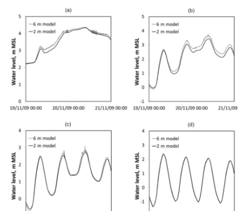
Finally, the highest-resolution 2 m model (CG02), fully em-bedded within CG06, covers the urban area of Cork city; this area is particularly prone to flooding. In the first step of model skill analysis, water elevations simulated by the CG06 and CG02 models at four locations along the river channel are compared in Fig. 13 and statistically summa-rized in Table 4. Again, the November 2009 flood event was used as a benchmark. Close to the east boundary, at point CG02_4 (see Fig. 14 for point location), both mod-els perform almost identically, and this is visually and sta-tistically confirmed in Fig. 13d and in Table 4, respec-tively. Discrepancies between the CG06 and CG02 models increase with distance from the nested east boundary and are manifested by overall higher water elevations computed by the coarser CG06 model. Location CG02_2 (Fig. 13b) shows the biggest discrepancy evidenced by the statistical measures RMSE=0.195 m, RMSD=0.109 m and RMSd-iff= −0.181 m. Despite overprediction of water elevations by the CG06 model, the general water level trends in the two models are in good agreement (COR=0.997). Another important advantage of a high-resolution model is an im-proved numerical stability of the model solution. As can be seen from Fig. 13a–c, some infrequent random oscillations in water levels occurring in CG06 from numerical instability due to insufficient grid resolution are not present in the finer CG02 model.
The numerical instability of the MSN_Flood model is di-rectly related to the grid resolution and results from an ADI
Figure 13.Time series of water elevations predicted by CG06 and CG02 at four locations:(a)CG02_1,(b)CG02_2,(c)CG02_3 and (d)CG02_4. Point locations shown in Fig. 14.
algorithm used in the model’s solution procedure. In general, the models using ADI are very accurate numerically in mod-elling flows; however, in the presence of a discontinuity, such as in regions of sharp gradients (e.g. velocity gradients, el-evation gradient or high elel-evations), the numerical models using such schemes are prone to generate spurious numer-ical oscillations (Kvoˇcka et al., 2015). A common solution used to reduce these oscillations is to increase the grid reso-lution so the slopes over numerical grids are milder. Compar-ing time series outputs from CG06 and CG02 (Fig. 13), it is evident that increasing resolution of the model significantly reduces numerical errors and hence oscillations.
The effect of improved horizontal resolution is analysed spatially by means of RET distribution plots. As shown in
Figure 14.Water level RET(%) in CG02 relative to SG02. Red dots denote points used in water level analysis (see Fig. 13).
between CG02 and SG02. In general, RET is quite low at
10 % in the western part of the city along river banks, in-creasing in eastward direction to 20 % in narrow streets of city centre. This is a considerable improvement when com-pared to RETin CG06 relative to SG02. Moreover, as CG02
achieves a similar level of accuracy to SG02, the computa-tional cost is significantly reduced and constitutes an enor-mous 96 % savings.
From this analysis it can be seen that the CG06–CG02 nesting results in a model performance generally comparable to the single-grid SG02 model but at a significantly reduced computational cost when compared to the single-grid model. The ultimate conclusion from the model validation is that MSN_Flood facilitates significant improvements in model accuracy without incurring the computational expense of high spatial resolution over the entire model domain. The model setup constitutes a rigorous test of model performance and on that basis it can be further concluded that the model is applicable to situations where nested boundaries are located in complex urban floodplains that periodically wet and dry. 3.2 Urban flood modelling
For most of the time, city streets are dry, and rivers drain-ing the hinterland are contained within well-defined river banks or walls. However, when extreme flood events occur, rivers may burst their banks and the city streets become water conveyance channels. The simulation of the hydrodynamics associated with rapid urban flood events is complex; many significant issues must be addressed such as flooding and drying, spatial resolution, domain definition, frictional re-sistance and boundary descriptions. When modelling flood events, the mathematical formulation of the nested bound-aries that permit flooding and drying is of particular impor-tance. Also, the horizontal resolution necessary to resolve small-scale processes must be considered. In particular, these aspects of the MSN_Flood model will be discussed in this section.
3.2.1 Extreme flood event
On 19 and 20 November 2009 high River Lee flows com-bined with high astronomical tides and moderate surge caused localized overtopping/breaching of the river banks, resulting in widespread flooding of Cork city. Evolution of the flood wave propagation simulated by the CG02 model is shown in Fig. 15. Maximum flooding was reached at 09:30 LT on 20 November 2009 around the time of high tide and approximately 5 h after peak discharge of River Lee. At this juncture over 62 ha of Cork city had been flooded. The most affected zone was the city centre located between the north and south channels of the river; this area is a low-lying island that over centuries was gradually reclaimed from marshland and its low-lying topography combined with the influence of river, estuary and harbour makes the area partic-ularly vulnerable to flooding.
Figure 15.Temporal evolution of flood wave through upper and lower floodplains of Cork city during the November 2009 flood event modelled by CG06; contours represent 2 h intervals.
Figure 16.Maps of flood inundation(a)observed by OPW and(b)modelled; contours represent 2 h intervals. Evolution of modelled flood wave is a combined output of CG06 and CG02.
as the model solution falls on the 45◦line. Interestingly, bet-ter agreement was found for survey locations in floodplains than at points adjacent to the river bank. This could be at-tributed to the fact that the majority of survey points are lo-cated away from the channel edge (many are actually at the floodplain edge).
3.3 Moving boundary
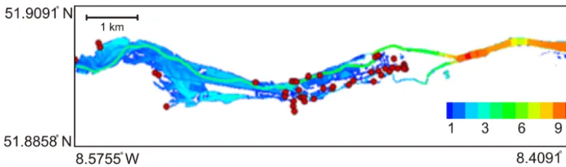
Figure 17.Maximum water levels during November 2009 flood event and water level survey points marked as red dots.
Figure 18.Comparison of modelled and observed maximum water elevations at 38 survey stations.
mathematical formulation of the nested boundary involving ghost cells, internal boundary formulation and adaptive in-terpolation ensures stable flooding and drying of boundary cells. In MSN_ Flood, any nested boundary can be placed within a flooding and drying zone and therefore may be sub-ject to significant lateral expansion and contraction. More-over, the internalization of the boundary allows the flood-ing and dryflood-ing mechanism to approach the boundary of the nested domain from either upstream or downstream. As the boundary alternatively floods or dries, the number of ac-tive boundary cells expands and contracts accordingly. De-pending on local topography, not only the length of the boundary may change, but also the number of active bound-aries changes. Such a boundary is therefore a complex, non-continuous, moving boundary that spatially and temporally changes its characteristics. This is a significant aspect of this research.
In the model setup, the urban CG02 model is entirely em-bedded within the CG06 model; mass and momentum from the 6 m model are transferred to the 2 m model via two nested boundaries – the western boundary, transferring River Lee waters from the upper to the lower channel of the river (it also geographically divides the floodplains into upper and lower
floodplains), and the eastern boundary, exchanging waters with the estuary. The western boundary of CG02 is located on the upstream fluvial floodplain, which is prone to wetting and drying. A cross section through this boundary illustrating the steep gradients of the river channel bathymetry and the to-pography of the adjacent urban floodplains (which includes buildings) is shown in Fig. 19. The temporal progression of water levels throughout the November 2009 flooding is also plotted. The reference water level at simulation timet=4 h corresponds to a 187 m3s−1river flow (19 November 2009 at 01:30). At this juncture the flow greatly exceeds the av-erage river flow of 40 m3s−1 as it results from increased discharges from Inniscarra Dam. The storage capacity of In-niscarra Reservoir had been reached after a month-long pe-riod of record-high rainfalls and heavy downpours on 18 and 19 November. Over the course of the subsequent 28 h the discharges further increased to reach a maximum value of 560 m3s−1at 02:30 on 20 November. The water level at the boundary increased from 4.57 m OD at 22:30 on 18 Novem-ber to a peak of 5.74 m OD 28 h later.
Figure 19.Cross section through west boundary of CG02 with wa-ter elevation marks for selected time points.
land; here the water elevation difference between two chan-nels is 0.31 m. This elevation difference further increases to 0.41 m near the nested boundary (cross section 3).
The temporal rise of water levels at a number of points across the western nested boundary is shown in Fig. 21. Se-ries A represents the main river channel, seSe-ries B and C cor-respond to points adjacent to the river channel, and series D is located in the side channel. The difference in water eleva-tions between the two boundaries is apparent throughout the entire flooding period, though it is reduced with the progress of flooding.
An interesting characteristics of the moving boundary is the change in its length. As flood waters continue overtop-ping the river banks, the area of inundation increases and is reflected in the elongation of the boundary. The length of the main channel boundary is initially equal to the river width; this nearly doubles during flooding as shown for t=12 h in Fig. 19. The temporal evolution of flooding through the boundary clearly demonstrates that the nested boundary is a discontinuous moving boundary with a variable head.
The numerical stability of such dynamically changing properties of nested boundary is an important aspect of nest-ing procedures. Overall, a change in length as well as di-vision into separate subsections does not markedly impact computational stability nor model performance. In fact, as shown in Fig. 14, RET computed over the flooding
pe-riod remain low within the CG02 domain despite significant changes to nested boundary configurations and flow condi-tions.
As demonstrated in this section, MSN_Flood has been de-veloped in a general-purpose manner that through stable and accurate moving boundary provides a high degree of choice and flexibility regarding the location of the boundaries to the nested domain.
Figure 20. (a)Flood extent in upper floodplains and(a–c)water elevations at three cross-sections during flood simulated by CG06.
3.4 Model resolution
Figure 21.Time series of water elevations across the western nested boundary of CG02.
Figure 22.Comparison of flood extent simulated by(a)CG02 and (b)CG06. Contours represent water levels (m).
Modelling of flood flow through an urban area is diffi-cult because of its need for stable and accurate solution of the flow equation (Brown et al., 2007). Since accurate mod-elling requires a resolution commensurate with flow features, dense street network flows through urban floodplains can only be fully resolved with a sufficiently high resolution. However, satisfactory model resolution, and thus accuracy, incurs computational expense; a balance between these two contradicting factors provides an optimal solution. Gallegos et al. (2009) found that a 5 m resolution mesh that spans a street by approximately three cells achieves such balance. The characteristics of urban residential areas of southern Cal-ifornian investigated in their study is different than that of an old European towns comprising narrow, dense streets as Cork city. It follows that the 5 m model resolution is insufficient to resolve flow dynamics in such city centre street networks.
Figure 23.Contour plots of(a)difference in water elevations (m) between CG06 and CG02, and(b)RMSE over time.
partic-Figure 24.Evolution of the relative difference in(a)total area of in-undation and(b)volume of water in inundated area between CG06 and CG02. See text for explanation of relative difference.
ular time. Figure 24a and b show the evolution of differences between CG02 and CG06 solutions in inundated areas and volumes throughout the simulation. The significantly high relative difference in the area at the initial stage of flood-ing reachflood-ing 36 % is misleadflood-ing as the relatively small total inundated area with a small flood time lag results in large discrepancies at this stage (ca. 11 ha). Nevertheless, when the flooding is more pronounced (over 30 ha, max 62.6 ha) the relative difference is still up to 10 %. With regards to flood water volume in inundated areas the difference is over 20 % during the first hours of flooding and still remains as high as 10 % throughout the flood peak, only falling to be-low 10 % when the flood recedes. The total RMSE of inun-dated area and volume between 2 and 6 m models is 3.4 ha and 21 367 m3, respectively. This comparison demonstrates that horizontal resolution is of paramount importance when simulating flows through complex topography. It seems that for Cork city centre, comprising a dense network of narrow streets, neither the 5m resolution requirement nor the three-cell street span would resolve complex flood flow at a satis-factory level of accuracy.
3.5 Flood water velocities
Another significant advantage of MSN_Flood is its ability to simulate the velocities of flood waters. As opposed to sim-plified 2-D hydraulic models frequently used in urban flood-ing, the hydrodynamic MSN_Flood includes both the conti-nuity and momentum equations, solving for both water el-evations and water velocities. Figure 25 shows an example of flood water velocities computed by MSN_ Flood in a se-lected area of Cork city centre blown up for ease of viewing; one can see flood waters in both the river channel and the urban floodplain. This zone is characterized by fast-flowing shallow water subject to rapid transitions as it flows down through the steep section of recreational grounds adjacent to the river channel. The city downtown, in contrast, is a pond-ing area with relatively stagnant waters.
Knowledge of velocity fields facilitates better understand-ing of flood water hydrodynamics and in particular the mech-anisms of flood propagation. The routes and speeds of flood
Figure 25.Map of velocity contours (m s−1) with vectors showing magnitude and direction of velocities in the downstream floodplains of Cork city.
waves provide important information for the evaluation of flood risks to people’s safety and to property, as well as to the planning and actions of emergency response teams.
4 Discussion
Inundation of coastal areas due to coastal and/or fluvial urban flooding mechanisms is a very complex hydrological phe-nomena, and developing a modelling system to accurately simulate it is not a trivial task. The research presented in this paper demonstrates that the concept of nesting models is very suitable for complex urban coastal flooding as they facilitate the development of an integrated system capable of resolving hydrodynamics at spatial scales commensurate with flows and physical features of the region of interest. The modelling system adopted here determines physical processes simulta-neously at different scales ranging from bay-size circulation (90 m) through mesoscale processes of coastal waters at 30 m resolution down to the ultra-high-scale environment of 2 m. Validation results show that the model performs well at each of these scales.
re-due to boundary formulation errors is commonly compen-sated by indirect solutions such as boundary configuration (e.g. location). For example, Kashefipour et al. (2002) in or-der to reduce possible nesting error dynamically link a 2-D coastal model with a 1-D river model by using overlapping grids at the boundary – a common area where boundary val-ues are exchanged between two models. Such a model setup is not required in MSN_Flood, where accurate exchange of boundary conditions occurs along a boundary.
Secondly, the model has virtually no limit to the number of specified nesting levels (and spatial resolution) and is primar-ily constrained by computational effort rather than numeri-cal stability. The highest resolution of 2 m set for this study was dictated solely by the resolution of available lidar data, and higher resolutions are easily achievable if suitable ter-rain data are available. For example, a 0.025 m resolution was used to simulate flows corresponding to those in a physical scale model of a harbour of dimensions 1.0×1.0×0.25 m (Nash and Hartnett, 2014). In this way, the model allows improved accuracy of solution when compared to a lower-resolution parent model where the improved accuracy is sim-ilar to that of a simsim-ilar high-resolution single-grid model, but the computational effort is significantly reduced.
Thirdly, the model provides adequate solutions at scales sufficient for processes of interest, such as coarse-resolution coastal circulation and fine-resolution flood inundation. This is attributed to the robust hydrodynamic module which in essence adopts the well-tested numerical scheme and dis-cretization methods described by Falconer and Chen (1991). The uniqueness and improvement of MSN_Flood over other nested models are its formulation of the nested boundary in the area where flooding and drying may occur. In order to ac-commodate flooding and drying of boundary cells, the model allows a moving nested boundary so that large sections of the boundary can alternatively wet and dry. The stable flooding and drying of boundary cells result from the internalization of the nested boundary combined with an adaptive interpola-tion technique tailored specifically for this model. To the au-thors’ knowledge the development of a non-continuous mov-ing nested boundary in a circulation model is novel. Such an innovative solution does not pose restrictions on the location of nested grids with regards to wetting and drying (as demon-strated by the application to Cork Harbour) and, therefore, allows flexibility of model setup.
Finally, in the context of urban flood modelling, MSN_Flood’s ability to simulate horizontal components of water velocity is a significant advantage over simpler hy-draulic models commonly used in flood modelling; the com-plexity of urban topography (buildings, vegetation, walls, roads, embankments, ditches etc.) necessitates at least two-dimensional treatment of surface flows (Cook and Merwade,
Although the modelling framework seems to be the main factor controlling accuracy of model predictions, other fac-tors such as model resolution, datasets and model parameter-ization also play a crucial role. In relation to model topog-raphy/bathymetry, these aspects are interconnected and need to be considered jointly. By comparing the 6 and 2 m grid models, it can be seen that results are quite sensitive to the spatial resolution of the model. The resolution acts as a filter on the model terrain so the model error increases with de-creasing spatial resolution, as the definition of topographic features (walls, hedges etc.) are progressively lost from the model bathymetry. There is a dual effect of this. Firstly, as the resolution becomes less granular, the high-density small features of topography become sub-grid phenomena, which then become parameterized through roughness coefficients. Spatially varying roughness needs to be specified for differ-ent terrains; this is determined based on surface classification (such as land type, vegetation or roads) within model sen-sitivity and calibration. Secondly, the loss of larger objects such as buildings makes the model inherently ill-conditioned, and their loss cannot be remedied through modification of roughness coefficient alone. Errors are additionally amplified by a presence of bias in the topographic data resulting from lidar-related post-processing difficulties such as representa-tion of surface objects as discussed in Mason et al. (2003).
5 Conclusions
In this research, high-resolution multi-scale modelling of coastal flooding due to tides, storm surges and rivers inflows is performed. The MSN_Flood modelling system is used to simulate flood water inundation of Cork city. The main find-ings from this research fall into two categories as follows:
1. Model computational performance:
a. The nesting model framework allows the model op-eration at practically any desired horizontal lution, including scales commensurate with reso-lution of lidar data making optimal use of such datasets: in the current setup, a four-nest cascade telescopes resolution down to the level of lidar res-olution, which is sufficient to capture small-scale flow features.
b. The model has no limits as to the number of nest-ing levels, and the numerical stability is maintained down to the finest resolution.
was found to be almost as accurate as a single-grid model of the same resolution but at a 96 % savings in computational cost.
d. Due to its robust flooding and drying routine, the model maintains numerical stability and accuracy in any part of the model domain affected by these processes.
e. Internalization of the nested boundary through the use of ghost cells combined with a tailored adap-tive interpolation technique permits flooding and drying of the nested boundary, creating highly dy-namic moving boundaries. Moreover, the flooding and drying mechanism can approach the bound-ary of the nested domain from either upstream or downstream. Nesting with a moving boundary al-lows embedding of a child grid model within the parent model in areas where the nested boundary may wet or dry. This unique feature of MSN_Flood provides a high degree of choice regarding the lo-cation of the boundaries to the nested domain and therefore flexibility in model application. This ca-pability gives MSN_Flood significant advantages over other models.
2. Model accuracy:
f. The modelling system demonstrates a good capa-bility to accurately determine physical processes at different spatial scales, including mesoscale coastal water circulation (90 m) and small scale hydrody-namics of complex urban floodplains (2 m). g. The extent of flood inundation into floodplains of
Cork city and maximum water levels reached dur-ing flooddur-ing were accurately simulated by the urban flood 2 m grid model.
h. Fine horizontal resolution is crucial for accurate as-sessment of inundation. Comparison of 6 and 2 m grid model RETin water levels shows a noticeable
reduction in model performance at coarser resolu-tion over the entire domain, and the error is gener-ally greater in the dense street network of an urban-ized zone.
i. The urban flood model provides full characteris-tics of water levels and flow regimes necessary for assessment of flood risk to people’s safety ated with particular flood water levels and associ-ated flood water velocities.
To conclude, near-unlimited model resolution, geographi-cally unconstrained (due to wetting and drying) nested model setup, robust wetting and drying routine, computational effi-ciency and the capability to simulate both water elevations and velocity fields make the MSN_Flood a valuable tool for studying coastal flood inundation. This research demon-strates that the adopted methodology can be successfully
used in applications to coastal flood modelling including complex urban environments. It can provide, at specific in-stances of time, accurate spatial distributions of water el-evations and flow magnitudes in inundated areas and can, thus, provide critical information to assess possible extents of flood inundation, periods of inundation, maximum wa-ter elevations reached, and flood wave propagation routes and speeds. Ultimately, it can be directly used for evalua-tion of flood risks to the area and indirectly, through some functional relationships, for risk assessment of human safety and property damage. The methodology explored in this re-search, when applied in a forecasting sense, constitutes a high-resolution flood warning and planning system that can aid local decision makers targeting high-flood-risk areas.
6 Data availability
Data to develop this model were made available by the Irish OPW. These data may be made available from OPW on re-quest from the corresponding author.
Acknowledgements. This publication has emanated from research conducted with the financial support of Science Founda-tion Ireland (SFI) under grant numbers SFI/12/RC/2302 and SFI/14/ADV/RC3021. The authors would like to thank OPW, Ireland for hydrological data and ECMWF for meteorological data. The authors would like to acknowledge the SFI/HEA Irish Centre for High-End Computing (ICHEC) for the provision of computational facilities and support. Useful suggestions from the two reviewers are appreciated.
Edited by: P. Tarolli
Reviewed by: two anonymous referees
References
Bates, P. D. and De Roo, A. P. J.: A simple raster-based model for flood inundation simulation, J. Hydrol., 236, 54–77, 2000. Bates, P. D., Dawson, R. J., Hall, J. W., Horritt, M. S., Nicholls,
R. J., Wicks, J., and Hassan, M. A. A. M.: Simplified two-dimensional numerical modelling of coastal flooding and exam-ple applications, Coast. Eng., 52, 795–810, 2005.
Bates, P. D., Horritt, M. S., and Fewtrell, T. J.: A simple inertia formulation of the shallow water equations for efficient two-dimensional flood inundation modelling, J. Hydrol., 387, 33–45, 2010.
Brown, J. D., Spencer, T., and Moeller, I.: Modeling storm surge flooding of an urban areas with particular reference to modelling uncertainties; A case study of Canvey Island, United Kingdom, Water Resour. Res., 43, W06402, doi:10.1029/2005WR004597, 2007.
guide, DHI water and Environment, 2001.
Falconer, R. A.: A mathematical model study of the flushing charac-teristics of a shallow tidal bay, P. Civil. Eng. Pt. 2, 77, 311–332, 1984.
Falconer, R. A. and Chen, Y. P.: An improved representation of flooding and drying and wind stress effects in a 2-D tidal nu-merical model, P. Civil. Eng Pt. 2, 91, 659–678, 1991.
Fewtrell, T. J., Duncan, A., Sampson, C. C., Neal, J. C., and Bates, P. D.: Benchmarking urban flood models of varying complexity and scale using high resolution terrestrial LiDAR data, Phys. Chem. Earth, 36, 281–291, 2011.
Formaggia, L., Gerbeau, J. F., Nobile, F., and Quarteroni A.: On the coupling of 3D and 1D Navier-Stokes equations for flow prob-lems in compliant vessels, Comput. Method. Appl. M., 191, 561– 582, 2001.
Gallegos, H. A., Schubert, J. E., and Sanders, B. F.: Two-dimensional high-resolution modelling of urban dam-break flooding: A case study of Baldwin Hill, California, Adv. Water Resour., 32, 1323–1335, 2009.
Gomes-Pereira, L. M. and Wicherson, R. J.: Suitability of laser data for deriving geographical data: a case study in the context of management of fluvial zones, Photogrammetry and Remote Sensing, 54, 105–114, 1999.
Haidvogel, D. B., Arango, H., Budgell, W. P., Cornuelle, B. D., Cur-chitser, E., Di Lorenzo, E., Fennel, K., Geyer, W. R., Hermann, A. J., Lanerolle, L., Levin, J., McWilliams, J. C., Miller, A. J., Moore, A. M., Powell, T. M., Shchepetkin, A. F., Sherwood, C. R., Signell, R. P., Warner, J. C., and Wilkin, J.: Ocean forecasting in terrain-following coordinates: Formulation and skill assess-ment of the Regional Ocean Modeling System, J. Comp. Phys., 227, 3595–3624, 2008.
Halcrow: Lee catchment flood risk assessment and management study, Hydrology report, Halcrow Group Ireland Ltd., 2008. Holt, J., Harle, K, Proctor, R., Michel, S., Ashworth, M., Batstone,
C., Allem, I., Holems, R., Smyth T., Haines, K., Bretherton, D., and Smith G.: Modelling the global coastal ocean, Philos. T. R. Soc. A, 367, 939–951, 2009.
Horritt, M. S.: Calibration and validation of a 2-dimensional finite element flood flow model using satellite radar imaginary, Water Resour. Res., 36, 3279–3291, 2000.
Horritt, M. S., Bates, P. D., and Mattinson, M. J.: Effects of mesh resolution and topographic representation in 2D finite volume models of shallow water fluvial flow, J. Hydrol., 329, 306–314, 2006.
Hunter, N. M., Bates, P. D., Neelz, S., Pender, G., Villanueva, I., Wright, N. G., Liang, D., Falconer, R. A., Lin, B., Waller, S., Crossley, A. J., and Mason, D. C.: Benchmarking 2D hy-draulic models for urban flooding, Water Management, 161, 13– 30, 2008.
Kashefipour, S. M., Lin, B., Harris, E., and Falconer, R. A.: Hydro-environmental modelling for bathing water compliance of an es-tuarine basin, Water Res., 36, 1854–1868, 2002.
Korres, G. and Lascaratos, A.: A one-way nested eddy resolv-ing model of the Aegean and Levantine basins:
implemen-events, Nat. Hazards, 79, 1791–1808, 2015.
Lin, B. and Falconer, R. A.: Tidal flow and transport modelling us-ing ULTIMATE QUICKEST scheme, J. Hydraul. Eng.-ASCE, 123, 303–314, 1997.
Mark, O., Weesakul, S., Apirumanekul, C., Aroonnet, S. B., and Djordjevic, S.: Potentials and limitations of 1D modelling of ur-ban flooding, J. Hydrol., 299, 284–299, 2004.
Marks, K. and Bates, P. D.: Integration of high-resolution topo-graphic data with floodplain flow models, Hydrol. Process., 14, 2109–2122, 2000.
Mason, D. C., Cobby, D. M., Horritt, M. S., and Bates, P. D.: Flood-plain friction parameterization in two-dimensional river flood models using vegetation heights derived from airborne scanning altimetry, Hydrol. Process., 17, 1711–1732, 2003.
Mason, D. C., Horrit, M. S., Hunter, N. M., and Bates, P. D.: Use of fused airborne scanning laser altimetry and digital map data for urban flood modelling, Hydrol. Process., 21, 1436–1447, 2007. McMillian, H. K. and Brasington, J.: Reduced complexity strategies
for modelling urban floodplan inundation, Geomorphology, 90, 226–243, 2007.
Nash, S.: Development of an adaptive mesh inter-tidal circulation model, PhD Thesis, Collage of Engineering and Informatics, Na-tional University of Ireland, Galway, 2010.
Nash, S. and Hartnett, M.: nested circulation modelling of inter-tidal zones: details of nesting approach incorporating moving bound-ary, Ocean Dynam., 60, 1479–1495, 2010.
Nash, S. and Hartnett, M.: Development of a nested circulation model: boundary error reduction, Environ. Modell. Softw., 53, 65–80, 2014.
Nittis, K., Perivoliotis, L., Korrea G., Tziavos, C., and Thanos, I.: Operational monitoring and forecasting for marine environmen-tal applications in the Aegean sea, Environ. Modell. Softw., 21, 243–257, 2006.
Olbert, A. I. and Hartnett, M.: Storms and surges in Irish coastal waters, Ocean Modell., 34, 50–62, 2010.
Olbert, A. I., Nash, S., Cunnane, C., and Hartnett, M.: Tide-surge interactions and their effects on total sea levels in Irish coastal waters, Ocean Dynam., 63, 599—614, 2013.
Olbert, A. I., Comer, J., Nash, S., and Hartnett, M.: High-resolution multi-scale modelling of coastal flooding due to tides, storm surges and river inflows. A Cork City example, Coast. Eng., 121, 278–296, doi:10.1016/j.coastaleng.2013.12.006, 2017.
Pappenberger, F., Beven, K., Horritt, M., and Blazkova, S.: Un-certainty in the calibration of effective roughness parameters in HEC-RAS using inundation and downstream level observations, J. Hydrol., 302, 46–69, 2005.
Pender, G. and Neelz, S.: Benchmarking of 2D hydraulic modelling packages. SC080035/R2 Environmental Agency, Bristol, p. 169, 2010.
Ponte, R. M.: Understanding the relation between wind- and pressure-driven sea level variability, J. Geophys. Res., 99, 8033– 8039, 1994.
Sanders, B. F., Schubert, J. E., and Detwiler, R. L.: ParBreZo: A par-allel, unstructured grid, Godunov-type, Shallow water code for high-resolution flood inundation modelling at the regional scale, Adv. Water Resour., 33, 1456–1467, 2010.
Simmons, A. J., Burridge, D. M., Jarraud, M., Girard, C., and Wergen, W.: The ECMWF medium-range prediction models de-velopment of the numerical formulations and the impact of in-creased resolution, Meteorol. Atmos. Phys., 40, 28–60, 1989. Smith, L. C.: Emerging applications of interferometric synthetic
aperture radar (INSAR) in geomorphology and hydrology, Ann. Assoc. Am. Geogr., 92, 385–398, 2002.
Spall, M. A. and Holland, W. R.: A nested primitive equation model for oceanic applications, J. Phys. Oceanogr., 21, 205–220, 1991. Uppala, S. M., Kallberg, P. M., Simmons, A. J., Andrae, U., Bech-told, V., Fiorino, M., Gibson, J., Haseler, J., Hernandez, A., Kelly, G., Li X., Onogi, K., Saarinen, S., Sokka, N., Allan, R., Anders-son, E., Arpe, K., Balmaseda, M., Beljaars, A., Berg, L., Bidlot, J., Bormann, N., Caires, S., Dethof, A., Dragosavac, M., Fisher, M., Fuentes, M., Hagemann, S., Holm, E., Hoskins, B., Isaksen, L., Janssen, P., McNally, A., Mahfouf, J., Jenne, R., Morcrette, J., Rayner, N., Saunders, R., Simon, P., Sterl, A., Trenberth, K., Untch, A., Vasiljevic ,D., Viterbo, P., and Woollen, J.: The ERA-40 reanalysis, Q. J. Roy. Meteor. Soc., 131, 2961–3012, 2005.
Yang, Z., Wang, T., Khangaonkar, T., and Breithaupt, S.: Integrated modelling of flood flows and tidal hydrodynamics over coastal floodplains, Environ. Fluid Mech., 12, 63–80, 2012.