http://www.sciencepublishinggroup.com/j/ajam doi: 10.11648/j.ajam.20180602.16
ISSN: 2330-0043 (Print); ISSN: 2330-006X (Online)
A New Method Detecting Abrupt Change Base on Moving
Cut Data-Permutation Entropy
Luo Wenxiang
1, Wan Li
1, 2, *, Lai Simin
11
School of Mathematics and Information Science, Guangzhou University, Guangzhou, China
2
Key Laboratory of Mathematics and Interdisciplinary Sciences of Guangdong Higher Education Institutes, Guangzhou University, Guangzhou, China
Email address:
*
Corresponding author
To cite this article:
Luo Wenxiang, Wan Li, Lai Simin. A New Method Detecting Abrupt Change Base on Moving Cut Data-Permutation Entropy. American Journal of Applied Mathematics. Vol. 6, No. 2, 2018, pp. 62-70. doi: 10.11648/j.ajam.20180602.16
Received: April 20, 2018; Accepted: June 6, 2018; Published: June 20, 2018
Abstract:
Permutation entropy is an effective index which can be used to describe the dynamic complexity of a time series, and it can effectively enlarge the small changes of a sequence. In this paper, the moving cut data-permutation entropy, a new method detecting abrupt change is raised by combining the permutation entropy method with the moving cut data technology. Different moving window scales are selected to analyze the mutational detection of linear and nonlinear time series via the new method respectively. The effect of peak noise and white Gaussian noise on this new method in nonlinear time series constructed by Lorenz equation and random sequence was studied. The results show that the moving cut data-permutation entropy method has strong anti-noise ability, which is able to precisely identify the mutational point of both the linear and nonlinear time series, and almost independent the scale of window and the length of sequence.Keywords:
Permutation Entropy, Moving Cut Data, Dynamical Structure, Mutational Detection1. Introduction
With the development of nonlinear science, sequence mutational detection technology has been developed rapidly. However, the traditional sequence mutational detection methods, such as Mann-Kendall, Yamamoto, Gramer method and sliding t-test, are highly dependent on the length of time series [1-3]. He in paper [4] given an example that the Mann-Kendall analysis of different length data of the same time series is completely different when using Mann-Kendall method to detect the nonlinear series. Due to the influence of the external force and the measurement error of the instrument, the nonlinear time series collected by the experiment is inevitably disturbed by all kinds of noise signals. Although the original data can be filtered the noise, it is impossible to eliminate the noise completely. Therefore, it is necessary to find a new method for detection that almost does not rely on sequence length and has a strong anti-noise ability.
Entropy is a measure of system complexity, developed rapidly after the establishment of information theory, which
hydrogeological system and medicine [13-26].
In this paper, the moving cut data-permutation entropy (MC-PE), a new method of dynamic structural mutational detection is raised by combining the permutation entropy method with the moving cut data technology, and the effectiveness and stability of the MC-PE method are verified by linear and nonlinear time series.
2. Methods
2.1. Permutation Entropy
Permutation entropy is an average entropy parameter to measure the complexity of one-dimensional time series put forward by Christoph Bandt. It is similar to Lyapunov exponent in terms of performance of time series complexity, but has the characteristics of simple operation and strong anti-noise ability. Permutation entropy is used to quantitatively characterize the complexity of a dynamic system which is more complex with the higher entropy and more regular with the lower entropy.
The basic principle of permutation entropy algorithm is as follows.
(i) Given a time series X = {x(n), n = 1, 2,⋯, N}, reconstructed the phase space of X and obtained the matrix is in the following:
(1) (1 ) (1 ( 1) )
( ) ( ) ( ( 1) )
( ) ( ) ( ( 1) )
x x x
x j x j x j
x K x
m
K x K
m m τ τ τ τ τ τ + + − + + − + + − ⋯ ⋮ ⋮ ⋮ ⋯ ⋮ ⋮ ⋮ ⋯
, j = 1, 2,⋯, K. (1)
K is the number of reconstructed vectors, K = N – (m – 1) τ, while m is called embedding dimension and τ is the delay time.
(ii) Each row in the reconstruction matrix rearranges in ascending order, defines the index for each element as permutation A (i) = ( j1,j2,
⋯
, jm ), that fulfills:x (i +(j1 – 1) τ) ≤ x (i + (j2 – 1) τ) ≤⋯≤ x (i + (jm– 1) τ) (2)
where i = 1, 2,
⋯
, N – (m – 1) τ. A simple example may help to clarify this concept. Assume a time series X = (3, 2, 5, 1, 4); for an embedding dimension of 3 and τ = 1, the first part would include the values (3, 2, 5). In order to rank these three values, the permutation (1, 0, 2) should be applied since1 2
t t t
x+ < <x x+ . Similarly, the second part (2, 5, 1) has the permutation type (2, 0, 1) with xt+2< <xt xt+1, and the third
arrangements. When Pi = 1/(m!), the permutation entropy PE
(m) gets the maximum value log (m!). As usual, log (m!) is used to normalize PE (m), that is
0 ≤ PE (m) = PE (m) / log (m!) ≤ 1 (4)
where PE (m) is consistent with the random degree of a time series X. Values of PE (m) close to one indicate the time series X with a stochastic dynamics, in which the elements in X are random. On the other hand, the PE (m) is closer to zero, the more fixed is the time series.
2.2. Moving Cut Data-Permutation Entropy
Moving cut data-permutation entropy is a mutational detection method formed by sliding removal technology on the basis of permutation entropy. The calculation process of MC-PE is as follows.
i) Choosing a window scale W of the slide removal data. ii) Removing data with length W continuously from time series {
x
(n), n = 1, 2,⋯
, N } and connecting the remaining N – W data, then a new subsequence of N – W is obtained.iii) Calculating the PE (m) by permutation entropy method. iv) Taking the slide step length to W, and moving the window gradually by keeping the window scale of data removed unchanged. It can get a PE (m) sequence with an int (N/W) length by repeating ii), iii) steps.
v) According the PE (m) sequence obtained from step iv), identifying the mutational point or mutational interval based on the data complexity is not very different in the same dynamic system, and it would be more distinct from different dynamic system.
3. Numerical Example
3.1. Mutational Detection of MC-PE Method in Linear Time Series
In order to test the effect of MC-PE method on dynamic structural mutational detection in linear time series, ideal linear time series (IS1) is constructed by the following equation [27]:
2 sin(0.3 ) 1, 1 1000,
( )
1.5 sin(0.3 ) 2 cos(0.8 ) 0.1, 1000 2000.
t t
y t =
t t t
+ ≤ ≤
+ − < ≤
(5)
Figure 1. Linear time series IS1.
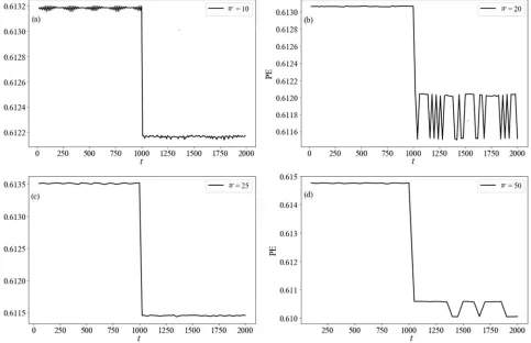
In this paper, the selection of permutation entropy parameters for all the ideal time series is m = 3, τ = 2. The MC-PE results of ideal linear time series IS1 in sliding removal window for W = 10, 20, 25, 50 are given in Figure 2, which show a similarity that the permutation entropy sequence obtained after removal of data are divided into two different stages with t = 1000 as the boundary. When t ≤ 1000, the values of permutation entropy are obviously greater than that at t > 1000 and the differences of the respective two evolutionary stages are almost negligible. According to the physical meaning of permutation entropy, the larger the entropy is, the greater complexity of the sequence. Therefore after removing the data, a smaller permutation entropy values mean that the data removed are more complex, which shows that the sequence complexity of t > 1000 is greater than the complexity of t ≤ 1000, fitting perfectly with the structure of IS1.
As shown in Figure 2 (b), a phenomenon similar to
periodic fluctuations occurred at t > 1000. The reason may be that the latter 1000 data of IS1 are determined by the cosine function of T = 20.94 (T is the period) and the cosine function of T = 7.85 at the same time, and the period of the sine function is very close to the slide removal window W = 20. In terms of the sine function, there are two situations for removing the last 1000 data from IS1 with window scale 20. The first one is that these 20 data are only affected by one period of the sine function and the second is that these 20 data are affected by the two periods of the sine function. Obviously, the first case is less complex than the latter, so the obtained entropy is a little bit higher to remove the first case than to remove the second one which shows that permutation entropy can effectively magnify the small change of time series. It can be easily determined that the ideal time series IS1 has a mutational point at t = 1001, and MC-PE method is suitable for dynamic structural mutational detection of linear time series.
(a) W = 10; (b) W = 20; (c) W = 25; (d) W = 50
[28-30]:
( )
x a x y
y xz cx y
z xy bz
= − −
= − + −
= −
ɺ
ɺ
ɺ
(6)
For the Lorenz system, taking the coefficient a = 10, b = 8/3, c = 28, the initial conditions (x0, y0, z0) = (0, 1, 0), and the step
length is 0.01 [31]. There are two strange attractors in the Figure 3 that means the system generated by Lorenz equations is chaotic. In other words, the sequence in Lorenz system is nonlinear. Particularly, the time series of variable z, ignoring the first 10000 data and choosing the next 1000 data, is selected as the research object, which is shown in Figure 4. On the other hand, the last 1000 data of IS2 is the random number that meets the standard normal distribution. In order to eliminate the dimension, standardizing the 1000 data came from Lorenz system before connecting two parts data is advisable.
Figure 3. Lorenz attractor.
Figure 4. The z-axis part time domain diagram.
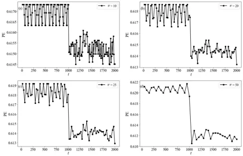
(a) W = 10; (b) W = 20; (c) W = 25; (d) W = 50
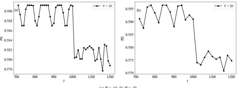
(a) W = 10; (b) W = 20
Figure 6. The MC-PE detection results of part nonlinear time series IS2.
The MC-PE results of ideal nonlinear time series IS2 in sliding removal window for W = 10, 20, 25, 50 are shown in Figure 5, which can be seen that the evolution trend of the permutation entropy values obtained by different sliding removal windows is very similar. The entropy values of the first half are higher than the second half, and this difference is very significant. The reason accounted for this difference is the complexity of the data in the second half of IS2 is significantly higher than that in the first half. Therefore, the permutation entropy is smaller when the data are removed at the second half of IS2 in same length. In other words, removing the data with high complexity makes the remaining data less complex, so the permutation entropy is smaller at t > 1000. As illustrated from Figure 5, the permutation entropy values are obviously distinct between t ≤ 1000 and t > 1000 in four different window scales,
and this distinction gradually increases with the increase of sliding removal window. Therefore, it can be judged that the mutational point of IS2 is about t = 1001.
To verify that whether the MC-PE method relies heavily on the length of the time series, 500 data is selected from IS2 between 700 to 1200. The MC-PE results are shown in Figure 6 revealing the same results as Figure 5, which means the detection result of MC-PE method is less dependent on the time series length.
The two common noises in the measured data are the peak noise and white Gaussian noise, so the effect of these two noises on the MC-PE method is tested. In the ideal time series IS2, the peak noise with the length of the original sequence is p = 10%, and the peak noise added is 5-6 times higher than the maximum value in the nonlinear time series IS2 (Figure 7) [32].
Figure 7. IS2 added p = 10% peak noise.
The value of peak noise and the position which should be added noise are selected randomly by computer. The mutational detection results of MC-PE when take p = 10%, W = 20, 25 are shown in Figure 8 (a) and (b), which found that the evolution of PE (m) values are bounded on two different states, and it can be clearly seen that the start time of the mutation, and the mutation point is about t = 1001. The PE (m) values obtained by MC-PE at t ≤ 1000 is significantly greater than that of t > 1000. It means that the dynamic structure changes at t = 1001, which is exactly the same as the actual dynamic structure of the ideal sequence IS2. In IS2, the first 1000 data are generated by the deterministic dynamics Lorenz equation, whose complexity is less than the latter 1000 random numbers. The PE (m) value after removing some of the more complicated random numbers is smaller, which is
completely consistent with the dynamic nature of the ideal sequence. It is indicated that the mutational detection result of MC-PE method is less affected by the peak noise.
(a) added p = 10% peak noise, W = 20; (b) just like (a), but W = 25; (c) added SNR = 19dB white Gaussian noise, W = 20; (d) just like (c), but W = 25
Figure 8. The MC-PE detection results of IS2 added noise.
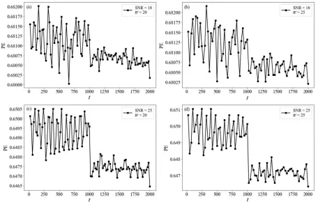
(a) SNR = 18dB, W = 20; (b) SNR = 18dB, W = 25; (c) SNR = 25dB, W = 20; (d) SNR = 25dB, W = 20
Through various numerical experiments, it finds that SNR = 18 dB is the SNR threshold which can detect the abrupt point. When SNR ≤ 18 dB, the clarity of the mutational point detected by the MC-PE method gradually decreased. On other hand, it gets the opposite result whose clarity is increasing when SNR > 18 dB. Keeping the window scale W = 20, 25 unchanged, the result of MC-PE of IS2 added white Gaussian noise with SNR = 18, 25 dB is given in Figure 9. When SNR = 18 dB, the PE (m) values in the first half are not always greater than the second part as SNR = 25 dB. Specially, the lowest point in Figure 9 (a) is at t = 660, not in the second part, which means the data near t = 660 is the most complex that is not consistent with the construction of IS2. Some points in the first half are still at a lower level, even if the sliding removal window increases to W = 25 in Figure 9 (b). But that's not the case when SNR = 25 dB,
which clearly shows PE (m) values change from a stable state to another stable state and the mutational point is at t = 1001. Compared Figure 8 and 9, it finds that the detection result of the abrupt change point becomes clearer with the increase of sliding removal window when signal-to-noise ratio at the same level.
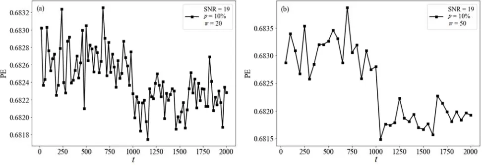
The measured data do not contain only one noise, they may contain two or more noises. So it is necessary to detect whether the MC-PE method still applicative when the data contains two kinds of noise. For the ideal time series IS2, the superposition is 10% of the original sequence, and the magnitude is 5-6 times of the maximum value in IS2 sequence and the white Gaussian noise with a signal-to-noise ratio of 19. It can see the MC-PE detection results of IS2 added mixed noise in Figure 10.
(a) SNR = 19dB and p = 10%, W = 20; (b) just like (a), but W = 50
Figure 10. The MC-PE detection results of IS2 added mixed noise.
Even if mixed with a high intensity of white Gaussian noise and peak noise, the results of MC-PE still show that PE (m) values are in two kinds of stable states, and also can be seen the two states near the boundary at t = 1000 clearly. The boundary becomes obvious as the slide removal window from W = 20 to W = 50. In simple terms, the detection result of MC-PE method is less influenced by white Gaussian noise and peak noise mixed. From what has been discussed above, the MC-PE method has a strong anti-noise ability.
4. Conclusion
Ideal time series analysis shows that the MC-PE method identifies the abrupt change point both the linear and nonlinear time series effectively. The location of the mutational point is detected precisely by MC-PE method and the detection result is almost not dependent on the window scale and the length of time series. The MC-PE method has strong anti-noise ability and its result is less influenced by the peak noise and white Gaussian noise even in a high noise level.
Acknowledgements
This work was supported by the National Natural Science Foundation of China (Grant No. 41172295); Innovation Research for the Postgraduate of Guangzhou University (2017GDJC-M32).
References
[1] A. B. Lüttger, and T. Feike. “Development of heat and drought related extreme weather events and their effect on winter wheat yields in Germany,” Theor. Appl. Climatol, Vol. 132, No. 1-2, 2017, pp. 1-15.
[2] T. Yamamoto, and M. Sano, “Theoretical model of chirality-induced helical self-propulsion,” Phys. Rev. E, Vol. 97, No. 1, 2018, pp. 012607.
regularity measure for fetal heart rate analysis,” Obstet. Gynecol., Vol. 79, No. 2, 1992, pp. 249-255.
[7] A. Singh, B. S. Saini, and D. Singh. “An adaptive technique for multiscale approximate entropy (MAE bin) threshold (r) selection: application to heart rate variability (HRV) and systolic blood pressure variability (SBPV) under postural stress.” Australas. Phys. Eng. Sci. in med., Vol. 39, No. 2, 2016, pp. 557-569.
[8] C. James, S. Azeem, S. Ric, B. Paul, and M. Chris, “Measurement of cardiac synchrony using approximate entropy applied to nuclear medicine scans,” Biomedical Signal Processing & Control, Vol. 5, No. 1, 2010, pp. 32-36. [9] S. M. Pincus, I. M. Gladstone, and R. A. Ehrenkranz, “A
regularity statistic for medical data analysis,” Journal of Clinical Monitoring, Vol. 7,No. 4, 1991, pp. 335–345. [10] L. Wan, X. Y. Hu, X. C. Deng, “Approximate entrop analysis
of metallogenic element content sequences and identification of mineral intensity: A case study of Dayingezhuang gold deposit,” Journal of China University of Mining & Technology, Vol. 43, No. 2, 2014, pp. 345-350.
[11] D. Y. Sun, Q. Huang, Y. M. Wang, Z. Liu, and L Zhang, “Application of moving approximate entropy to mutation analysis of runoff time series,” Journal of Hydroelectric Engineering, Vol. 33, No. 4, 2014, pp. 1-6.
[12] J. S. Richman, J. R. Moorman. “Physiological time-series analysis using approximate entropy and sample entropy,” Am. J. Physiol. Heart Circ. Physiol., No. 278, No. 6, 2000, pp. 2039-2049.
[13] D. E. Lake, J. S. Richman, M. P. Griffin, and J. R. Moorman, “Sample entropy analysis of neonatal heart rate variability,” Am. J. Physiol. Regul. Integr. Comp. Physiol. Vol. 283, No. 3, 2002, pp. R789- R797.
[14] F. Kaffashi, R. Foglyano, C. G. Wilson, and K. A. Loparo, “The effect of time delay on approximate & sample entropy calculations,” Physica D Nonlinear Phenomena, Vol. 237, No. 23, 2008, pp. 3069-3074.
[15] C. Bandt, and B. Pompe, “Permutation entropy: A natural complexity measure for time series,” Physical Review Letters, Vol. 88, No. 17, 2002, pp. 174102.
[16] M. Zanin, L. Zunino, O. A. Rosso, and D. Papo, “Permutation entropy and its main biomedical and econophysics applications: a review,” Entropy, No. 14, No. 8, 2012, pp. 1553-1577.
[17] M. Riedl, A. Müller, and N. Wessel. “Practical considerations of permutation entropy,” Eur. Phys. J. Special Topics, Vol. 222, No. 2, 2013, pp. 249-262.
[18] H. Azami, and J. Escudero. “Improved multiscale permutation entropy for biomedical signal analysis: Interpretation and application to electroencephalogram recordings,” Biomedical Signal Processing & Control, Vol. 23, No. 1, 2015, pp. 28-41.
[21] Y. Hou, F. Liu, J. Gao, C. Cheng, and C. Song, “Characterizing complexity changes in chinese stock markets by permutation entropy,” Entropy, Vol. 19, No. 10, 2017, pp. 514.
[22] Y. S. Choi, “Improved multiscale permutation entropy measure for analysis of brain waves,” International Journal of Fuzzy Logic & Intelligent Systems, Vol. 17, No. 3, 2017, pp. 194-201.
[23] O. Dostál, O. Vysata, L. Pazdera, A. Procházka, J. Kopal, J. Kuchyňka, and M. Vališ, “Permutation entropy and signal energy increase the accuracy of neuropathic change detection in needle EMG,” Computational Intelligence & Neuroscience, Vol. 2018, No. 6, 2018, pp. 1-5.
[24] M. Kuai, G. Cheng, Y. Pang, and Y. Li, “Research of planetary gear fault diagnosis based on permutation entropy of CEEMDAN and ANFIS,” Sensors, Vol. 18, No. 3, 2018, pp. 782.
[25] Y. Gao, F. Villecco, M. Li, and W. Song, “Multi-scale permutation entropy based on improved LMD and HMM for rolling bearing diagnosis,” Entropy, Vol. 19, No. 4, 2017, pp. 176.
[26] K. Keller, T. Mangold, I. Stolz, and J. Werner, “Permutation entropy: New ideas and challenges,” Entropy, Vol. 19, No. 3, 2017, pp. 134.
[27] Q. G. Wang, Z. P. Zhang, “The research of detecting abrupt climate change with approximate entropy,” Acta Phys. Sin., Vol. 57, No. 3, 2008, pp. 1976-1983.
[28] J. Guckenheimer, and R. F. Williams. “Structural stability of Lorenz attractors.” Publications Mathématiques De Linstitut Des Hautes Études Scientifiques, Vol. 50, No. 1, 1979, pp. 59-72.
[29] I. Grigorenko, and E. Grigorenko, “Chaotic dynamics of the fractional Lorenz system,” Physical Review Letters, Vol. 91, No. 3, 2003, pp. 034101.
[30] N. C. Kakwani, “Applications of Lorenz curves in economic analysis,” Econometrica, Vol. 45, No. 3, 1977, pp. 719-727. [31] P. G. Baines, “Lorenz, EN 1963: Deterministic nonperiodic
flow. Journal of the Atmospheric Sciences 20, 130-41,” Physical Geography, Vol. 32, No. 4, 2008, pp. 475-480. [32] H. M. Jin, W. P. He, W. Zhang, A. X. Feng, and W. Hou,
“Effect of noises on moving cut data-approximate entropy,” Acta Phys. Sin., Vol. 61, No. 12, 2012, pp. 069201-160. [33] I. Castillo, and R. Nickl. “Nonparametric Bernstein-von Mises
theorems in Gaussian white noise,” Annals of Statistics, Vol. 41, No. 4, 2013, pp. 1999-2028.
[35] S. S. Dasgupta, V. Rajamohan, and A. K. Jha, “Dynamic characterization of a bistable energy harvester under Gaussian white noise for larger time constant,” Arabian Journal for Science & Engineering, 2018, pp. 1-10.
[36] A. Dechant, A. Baule, and S. I. Sasa, “Gaussian white noise as a resource for work extraction,” Physical Review E, Vol. 95, 2017, pp. 032132.
[37] S. Benkrinah, and M. Benslama “Acquisition of PN sequences
using multilayer perceptron neural network adaptive processor for multiuser detection in spread-spectrum communication systems,” International Journal of Numerical Modelling Electronic Networks Devices & Fields, Vol. 31, No. 1, 2018, pp. e2265.