A MULTIVARIATE WEIBULL DISTRIBUTION

Cheng K. Lee

Loss Forecasting

Home Loans & Insurance Bank of America

Charlotte, North Carolina 28244 USA

[email protected]

Miin-Jye Wen

Department of Statistics

National Cheng Kung University Tainan, Taiwan 70101

Republic of China

Abstract

A multivariate survival function of Weibull Distribution is developed by expanding the theorem by Lu and Bhattacharyya. From the survival function, the probability density function, the cumulative probability function, the determinant of the Jacobian Matrix, and the general moment are derived.

Keywords: general moment; multivariate survival function; set partition; Weibull distribution; Copula; competing risks.

1. Introduction

Lu and Bhattacharyya (1990) developed a joint survival function by letting h x₁

 

and h₂

 

y be two arbitrary failure rate functions on



0,



, and H₁

 

x and H₂

 

y

be their corresponding cumulative failure rate. Given the stress S=s> 0, the joint survival function conditioned on s, as they defined, is

 

 



1 2



( , | ) exp

F x y s  _H x H y _ s ,

where  measures the conditional association of X and Y. Further, based on the joint survival function, they proved a theorem that a bivariate survival function

( , | )

F x y s can be derived with the marginalsFxandFygiven the assumption that the Laplace transform of the stressS exists on



0,



and is strictly decreasing.

From the theorem, they derived a bivariate Weibull Distribution

1 2

1 2

( , ) exp x y

F x y



 

 

 

 _{ } 

   

 _{ } 

 __{ } _{   }

   

 _{ } 

 

where0 <   1, 0 < 1, 2 < , and 0 < γ1, γ2 < . This bivariate Weibull

Following the same steps, the theorem can be expanded to more than two random variables, and, therefore, a multivariate survival function of Weibull distribution is constructed as

1 2

1 2

1 2

1 2

( , ,..., ) exp ...

n n n

n

x

x x

S x x x

 

 



 

  

 _{ } 

 

   

 _{ } 

 __{ } _{ }  _{   }

     

 _{ } 

 

(1)

where



measures the association among the variables, 0 < α ≤ 1, 0 < 1,2,…,n

< , and 0 < γ1,γ2,…,γn<.

This model can also be derived by using a copula construction with the generator

 





1/

log . 

 (Frees and Valdez 1998). Equation (1) is similar to the “genuine multivariate Weibull distribution” developed by Crowder (1989) who, in his paper, studied another version extended from the genuine multivariate Weibull distribution.

In this paper, we mathematically intensively studied the proposed multivariate Weibull model of Equation (1) by providing the probability density function, and the Jcaobian matrix in section 2, the general moment in section 3, an application in section 4 and conclusions in section 5.

2. Probability Density Function of The Multivariate Weibull Distribution

The multivariate probability density function f x x( ,_{1 2},...,x_n)of a multivariate distribution function can be obtained by differentiating the multivariate survival function with respect to each variable. Li (1997), and Yi and Weng (2006) had shown that:

1 2

( , ,..., _n)

f x x x =

 

1 2

1 2

( , ,..., )

1

...

n

n _n

n

S x x x

x x x

 

   .

Using Li’s derivation and one of the special cases of the multivariate Faa di Bruno formula by Constantine and Savits (1996), the probability density function is

1 2

1 2

1 2

1 2

1

( , ,..., ) exp ...

n n

n n

n

x

x x

f x x x

 

 



 

   

 _{ } 

 

   

 



  _{ }

_{  }_{ } _{ }  _{   }

   _      _ 

 

1 ₁ 2 _{1 1}

1 2 1 2

1 2 1 2

... ...

n

n n

n n

x

x x



 



 

  

     



 

 

    _      _

    _      _

          

 _{  }

 

 

  1 2

1 2

1 1 1 2

1 , ...

i n i

j i

k n

P n k

n

k _n

s

i j n

x

x x

P n i

 

 



 



  



 

 _{ } 

       

 _{ } 

 _  _{  } _{ }  _{   }

     

 

 _{ } 

 

wherekiis the number of summands of the ith partition of n such that

1 2 ki

n n n n, _{1 2} 0

i k

n n n  ,1k_i n;nj

is equal to



1 ...





n_j 1



      , the falling factorial of



(Kunth 1992);P n

 

is the total

number of partitions of n; P n i_s

 

, is the total number of set partitions of the set

n

S ={1,…,n} corresponding to the ith partition of n. The specific way of partitioning n andSnis given by McCullagh and Wilks (1988). In their paper, partitions of n are in increasing number of summands and ordering all the summands in inverse lexicographic order when a partition has the same number of summands, and S_n= {1,…, n} is partitioned by “listing the blocks from the largest to the smallest and by breaking the ties of equal sized blocks by ordering them lexicographically” and the number of blocks in a set partition is equal to the number of summands of the corresponding partition of n. For example, the total number of blocks of the partition ofSncorresponding to the i

th

partition iskiand the numbers of elements in each block are equal ton n1, 2,,nk_i.

Similar to the derivation of the Bivariate Weibull Distribution by Lu and Bhattacharyya (1990), let



y y1, 2,...,yn



= 1 2 1





1 2

1 2 1 2 1 2

, ,..., , ...

... ... ...

n

n

n n n

z

z z

z z z

z z z z z z z z z





 

  

 _{        } 

  (3)

where

1

1 1

1

x z

 



    

  ,

2

2 2

2

x z

 



 

  

  ,…,

n n n

n

x z

 



 

  

  .

Then, 1 1

1 1 1 n 1

x y y

  



 , 2 2

1 2 2 n 2

x y y



 



 ,…, 1 1

1

1 1 1

n n

n n n n

x y y



  



    ,



1 1 2 1



1

n n

n n n n

x y y y y

 

 



    _ .

Note that z1,z2,...,zn0, and

1 2 1

1 y y  ... y_n

= 1 2 1

1 2

... 1

...

n n

z z z

z z z



   

  

=

1 2 ...

n n

z

The Jacobian matrix is

J=

1 1 1

1 2

2 2 2

1 2

1 2

n

n

n n n n

x x x

y y y

x x x

y y y

x x x

y y y

  

  

  

  

  

  





  



.

LetC(i,j) be theithrow and jthcolumn in the Jacobian matrix, then

C(i,i)=

1 1

i i

i i n i

y y



 

 



,i=1,2,…,n-1,

C(i,n)=

1 1

i i i i n

i

y y

  

 



,i=1,2,…,n-1,

C(n,i)=





1 1

1 2 1

1 n

n

n n n

n

y y y y

  





 

   

  ,i=1,2,…,n-1,

C(n,n)=





1 1

1 2 1

1 n

n

n n n

n

y y y y

  





 

   _

, C(i,j)=0 whenij,i=2,…,n-1,j=2,…,n-1.

The determinant of the Jacobian matrix can be obtained using Gaussian elimination to construct an upper triangle matrix. The determinant is then equal to the product of the diagonal elements and is given as

|J| =

 

 

   

 

1 1

1 1

, ,

, ,

,

n n

j i

C n j C j n C i i C n n

C j j

 

 

 

 



 

 _{ }





_



_

=





1

1 1 2

1 2

1 1 1

1 1

1 1 1

1 2 1 2 1 1 2 1

1 2

1 n

n n

n

n n n n

n

y y y y y y y

 



 

   

 

   

  

 

    

  

     



  

 . (4)

After the derivation of the Jacobian, the PDF in terms ofy y1, 2,,yn,



1, 2, , n



g y y  y =





1 1

1 1 2 2

1 1

1 1

1 1, 2 2, , 1 1, 1 1 2 1

n n n

n

n n n n n n n n

f y y y y y y y y y y J



  _

  

  _   _  _{  }

  

 

   

 

 

=

 

 

 

( )

1 1

1 1

1 1 , exp( )

i j i i k P n n

n _k k

n s n

i j

y P n i y

             _   _       







=



 

1 1 1 1 1 1





1 1



1 2 ... n 1 1 1 2 ... n 1 ( n)

n y  y  y _  y y y _  f y

     , (5)

wherey₁,y₂,…,y_n1has a Dirichlet distribution with the probability density equal to

 

_{1 1 1 1 1 1}





1 1

1 2 ... n 1 1 1 2 ... n 1

n y  y  y _  y y y _ 

     , and

( _n)

f y =

 

 

 

 

( ) 1 1 1 1 1

1 , exp( )

i j i

i

n _{P n k}

n k

k

n s n

i j

y P n i y

n  

          _  _    _  _

 _



_{ }



_ (6)

has a mixture distribution of the exponential distribution and Gamma distribution. Equation (6) can be rewritten as:

( _n)

f y =

 

 

     

 

( )

1 1

1 1

1 exp( )

1 ,

i j i

i

n _{P n k}

n k

k n

n i s

i j i

y

y k P n i

n   k

           _{ }      _  _   _



_{ }



_  _ .

When it is integrated over the range of yn, it becomes:

 

 

     

( ) 1 1 1 1 1 , i j i

n _{P n k}

n k

i s

i j

k P n i

n  

         _{ }     _  _

 _



_{ }



_=1.

That is the weights ofynare summed to 1. The probability density function of ynis

the mixed Gamma distribution by Downton (1969). Following his derivation, the cumulative density function ofynis:

 

 

 

     

1 ( ) 1

1 1

1

1 1 , j exp( )

n _{n i P n k} n k

n

s n

i k i j

y

k P n i y

n i  

           _ _{ } _    __     









 . (7)

3. The General Moment

The general moment ofx x₁, ₂,,x_nis 1 2 1 2 n i i i n

E x x_ x _=





1

1 2

1 1

1 1 2 2

1 1

1 1

1 1 2 2 1 1 1 1 2 1

n n

n n n

n

i i

i i

n n n n n n n n

E y y y y y y y y y y

   _      _   _{   }       _{       }  _{           }          _{       }     

=



1 2



1 2 n i i i n   





1 1 2 1 1 2

1 2 1 1 1 2 1

n n n n i i i i n n

E y y y y y y

   _     _                 1 2 1 2 n n i i i n

E y   

Considering the second factor,





1 1 2 1 1 2

1 2 1 1 1 2 1

n

n n

n i

i i _i

n n

E y y y y y y

   _     _                 =

 





1 1 2 1 1 2

1 2 1 1 2 1 1 1

... 1 n n n n i

i i _i

n n n

n y y y y y y dy dy

   _    _{ }    

 

      =

 

1 2

1 2

1 2 1 2

1 1 n 1

n n n i i i n i i i n                  _  _{ }  _ _  _           _{ }    _ _      

which is the Dirichlet integral (Rao 1954)

For 1 2 1 2 n n i i i n

E y   

          

, let 1 2 1 2

n n

i

i i











=c, then

c n

E y_ _

=

 

 

 

 

( ) 1 1 1 1 0 1

1 , exp( )

i j i

i

n _{P n k}

n k

k c

n n s n n

i j

y y P n i y dy

n





          _  _    





_{ }



_ =

 

 

 

 

( ) 1 1

1 1 ₀

1

1 , exp( )

i j

i _i

n _{P n k}

n

k _{c k}

s n n n

i j

P n i y y dy

n  

           _{ }         



_{ }



_



_ =

 

 

 

 





( ) 1 1 1 1 1 , i j i

n _{P n k} n k

s i

i j

P n i c k

n





               



_{ }



_{ } =

 

 

 

 

 

( ) 1 1 1 1 1 , i j i i

n _{P n k} n

k _k

s

i j

P n i c c

n





             





_{ }



_{ } (8)

where _cki_{is the rising factorial defined as}



₁

 

₁



i

c c  c k by Knuth (1992). ConsideringP n i_s

 

, in the above equation, it is the total number of set partitions corresponding to the ithpartition ofn such that _{1 2}

i k

n n n n,n₁,n₂,…, i k

n >0.

It has been shown by McCullagh and Wilks (1988) that

 

,

s

P n i =

1 2 1 2

!

! ! ! ! ! !

i

k d

n

n n n m m m

Then, the product

 

1

,

i j k

n s

j

P n i





 

 







=

1 2 1 2

!

! ! ! ! ! !

i

k d

n

n n n m m m

1 2 nki n n   

=

1 2

!

! ! _d!

n

m m m ₁



₁



₂



₂







! ! !

! ! ! ! ! !

i k k

n n n n n n













 





=

1 2

!

! ! _d!

n

m m m n1 n2 nki 

   

  

 

  

    

= !

!

i

n

k _{1 2}

!

! ! !

i d

k

m m m n₁ n₂ nk_i 

   

  

 

  

    ,

where

1 2

!

! ! !

i d

k

m m m is the number of permutations ofn n1, 2,,nkiof every possible order.

When sum

 

1

,

i j k

n s

j

P n i





 

 





over the same value ofki, say, k, then,

 

1

,

i j

i

k n s

k k j

P n i



 

 

 

 





=

1 2 1 2

! !

! ! ! ! _i

i

i

k k k i d

k n

n

n n

k m m m

  



     

     

     

 







= !

!

n

k 1 2 1 2

!

! ! !

i

k k d k

k

n

n n

m m m

  



     

     

    

 







which equals C n k



, ,





, the C-numbers defined by Charalambides (1977). Note that the summation is over all the permutations of

i k

n withki=k.

Using the equality

 

1 ki k_i

 

ki

c c

   (Goldman, Joichi, Reiner and White 1976),

c n

E y_ _

=

 

 

 

 

 

( ) 1

1 1

1

1 ,

i j

i _i

n _{P n k} n

k k

s

i j

P n i c c

n







 

   



 

   

=

 

 

 

 

 

( ) 1 1 1 1 , i j i

n _{P n k}

n k s

i j

c P n i c

n  

         _  _         _



_{ }



_{ } =

 

 

1

 

1

 

1

 

1

,

i

j i

i

n _{n k}

n k s

k k k j

c P n i c

n





           _  _      _   _   _

 

_{  }



_{ } =

 

 

1

 

1



 

1

, ,

n _n

k k

c C n k c

n  

   _{ }  _  _ 



=

 

 

1

 



1 n n

c c

n  





 

 (using equation 1.3 by Charalambides 1977)

=

 

 

1

    

1

1

n

n n

c c

n  





 

 (using the formula by Goldmanet al. 1976)

=

  

1n



c1





c2

 



c   n 1

 

c 1



  .

Therefore, the general moment of x x1, 2,,xn is 1 2 1 2 n i i i n

E x x_ x _

=





1 1 2

1 2

1 1 2

1 2 1 2

1 2 1 2 1 1 1 2 1

n n

n

n n n

n

i i i i

i i

i i

i i

n E y y yn y y yn E yn

   _       _

 



                             

= 1 2

1 2 n i i i n   _

 

1 2

1 2

1 2 1 2

1 1 n 1

n n n i i i n i i i n                  _  _{ }  _ _  _           _{ }    _ _      

 

11 22 11 22

1

. n 1 n 2

n n

i i

i i i i

n        

                         _{ }  _{   }  _{ }…





1 2 1 2 1 n n i i i n                       1 2 1 2 1 n n i i i         _{ }    _ _      =

1 2 1 2 1 2

1 2

1 2 1 2

1 2 1 2

1 1 1 1

1

n i

i i n n

n

n n

n n

i i

i i i i

From the general moment, the expectation and the variance of any random variable, and the covariance and the correlation coefficient of any pair of variables can be derived. However, as Lu and Bhattacharyya (1990) pointed out, the correlation coefficient is non-negative.

4. Application

For illustration purpose, we fit the proposed model mode with n=3 to the data of Campbell and McCabe (1984). The data contains GPA, SAT (both math ban verbal) of 234 freshmen that majored in computer science. The data was downloaded from www.math.aau.dk/~s0ren/BusinessStatistics/data.html. Campbell and McCabe (1984) had shown that GPA is positively correlated with SAT’s math score and verbal score. Let GPA be X1, SAT math score be X2, and

SAT verbal score beX3. The PDF of the trivariate Weibull is

1 2 3

( , , )

f x x x

=

 

3

3 _{1 2 3} 1 2 3

( , , )

1 S x x x

x x x

 

  

=

3

1 2

1 2 3 1 2 3

2

1 2 3 1 2 3

x

x x

exp x x x

 

 



 

  

   

 _{ } 

 _      _ 

 _{ } _{    }

 _{ } 

     

 

 _{ } 

 

×

3 3

1 2 1 2

3

3 3

1 2 1 2

1 2 3 1 2 3

x x

x x x x



 

   

 

   













 

 

   

    _    _

 

   

    _    _

      _      _

×

3

1 2

3

1 2

1 2 3

2 3 1 x x x

 

 



 









 _{ } 

 _      _ 

 _ _{ } _{      }

     

 

 _{ } 

 

    

+

3 3

1 2 1 2

2

2 1 2 3 1 2 3

1 2 3 1 2 3

1 3 x x x x x x

 

 

   

 

   



     

   

   

       

 _{ }  _ _{ } 

   

       

_{   }  _ 

 

 



 

 

 _   _ _      _{ }



.

Let n denote the number of observations, then, the log-likelihood function becomes







1 2 3



1

log , ,

i i i

n i

f x x x





= 1 2 3

1

2 1 2 3

log

i i i n

i x x x

    

 

 

 

 



−

3

1 2

1 2 3

1 2 3

1

i i i

n i

x x x

 

 

  









_{     } 

 _{ } 

     

_{     } 

 

 

+

3 3

1 2 1 2 3

1 2 3 1

1

2 3

1 2 3 1 2 3

log i i i i i i

n i

x x x x x x



 

   

     

     

 



 

      _      _

 

      _      _

 

 

 

 

             



+

3

1 2

1 2 3

1 2 3

1

log 2 3 1 i i i

n i

x x x

 

 

  











 _{ } 

 _      _ 

 _ _{ } _{ } _{   }

     

 

 _{ } 

 

    



+

3 3

1 2 1 2

2

1 2 3 1 2 3

2

1 2 3 1 2 3

1 3 xi xi xi xi xi xi

 

 

   

     



     

   

           

_{     }  __{     } 

_{  }   

 

 



  

 

 _ _        



  



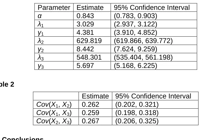
The parameters are estimated by maximizing the likelihood function, and the standard deviation for 95% confidence interval are approximated using the inverse of the negative Hessian of the log-likelihood function. The results of the fitted trivariate Weibull model are in Table 1.

After the parameter estimates are obtained, the covariance (denoted by Cov) and the variance (denoted by Var) can be calculated using the general moment of Equation 9.

The correlation coefficient betweenX1andX2is





 

 

1 2

1 2

,

Cov X X

Var X Var X

=



 

 









 







1 1 0 1 0 0 0 1 0

1 2 3 1 2 3 1 2 3

2 0 0 2 1 0 0 0 2 0 2 0 1 0

1 2 3 1 2 3 1 2 3 1 2 3

E X X X E X X X E X X X

E X X X E X X X E X X X E X X X



 

=0.262.

Repeatedly, the correlation coefficient between X1 and X3, X2 and X3 are

calculated. Table 2 shows the correlation confidents and their 95% confidence intervals of the 3 pairs of the random variables. The confidence intervals are calculated using Fisher’s z transformation formulas (Krishnamoorthy andXia 2007).

Note that when α equals 1, X1, X2 and X3 are independent. The estimate of α in

Table 1

Parameter Estimate 95% Confidence Interval

α 0.843 (0.783, 0.903)

λ1 3.029 (2.937, 3.122)

γ1 4.381 (3.910, 4.852)

λ2 629.819 (619.866, 639.772)

γ2 8.442 (7.624, 9.259)

λ3 548.301 (535.404, 561.198)

γ3 5.697 (5.168, 6.225)

Table 2

Estimate 95% Confidence Interval Cov(X1,X2) 0.262 (0.202, 0.321)

Cov(X1,X3) 0.259 (0.198, 0.318)

Cov(X2,X3) 0.267 (0.206, 0.325)

5. Conclusions

In this paper, we proposed a multivariate Weibull model that is similar to the genuine multivariate Weibull one by Crowder (1989). We further derived the explicit form of PDF, CDF, and the general moment. The explicit forms of these functions are desirable for numerical computations. We believe that the proposed model is a candidate for, first, testing the overall association on a given number of random variables that are Weibull distributed. It also becomes a competing risks model when the random variables in the proposed model are survival times to the corresponding events that, in business and management, could be paying off a loan, defaulting a loan, leaving a company, etc.

Acknowledgement

The authors thank Mr. Daniel Warren Whitman for proofreading the article.

References

1. Campbell, P. F. and McCabe, G. P. (1984). Predicting the Success of Freshmen in a Computer Science Major. Communications of the ACM 27: 1108-1113.

2. Charalambides, CH. A. (1977). A New Kind of Numbers Appearing in The n-Fold Convolution of Truncated Binomial and Negative Binomial Distributions. SIAM Journal on Applied Mathematics 33:279-288.

3. Constantine, G. M., Savits, T. H. (1996). A Multivariate Faa Di Bruno Formula with Applications. American Mathematical Society 358:503-520. 4. Crowder, M. (1989). A Multivariate Distribution with Weibull Connections.

Journal of the Royal Statistical Society, Series B 51:93-107.

6. Downton, F. (1969). An Integral Equation Approach to Equipment Failure. Journal of the Royal Statistical Society, Series B 31:335-349.

7. Frees, E. W., Valdez, E. A. (1998). Understanding Relationships Using Copulas. North American Actuarial Journal 2:1-25.

8. Goldman, J. R., Joichi, J. T., Reiner, D. L., White, D. E. (1976). Rook Theory. II, Boards of Binomial Type. SIAM Journal on Applied Mathematics 31:618-633.

9. Hougaard, P. (1986). A Class of Multivariate Failure Time Distributions. Biometrika 73: 671-678.

10. Knuth, D. E. (1992). Two Notes on Notation. The American Mathematical Monthly 99:403-422.

11. Krishnamoorthy, K. and Xia, Y (2007). Inferences on Correlation Coefficients: One-Sample, Independent and Correlated Cases. Journal of Statistical Planning and Inference 137: 2362-2379.

12. Li, C. L. (1997) A Model for Informative Censoring. Ph.D. Dissertation: The University of Alabama at Birmingham.

13. Lu, J-C., Bhattacharyya, G. (1990). Some New Constructions of Bivariate Weibull Models. Annals of the Institute of Statistical Mathematics 42: 543-559.

14. McCullagh, P. M., Wilks, A. R. (1988). Complementary Set Partitions. Proceeding of the Royal Society of London 415: 347-362.

15. Rao, S. K. L. (1954). On the Evaluation of Dirichlet’s Integral. The American Mathematical Monthly 61:411-413.