Muhammad Aslam
Department of Statistics Quaid-i-Azam University Islamabad, Pakistan [email protected]
Ghausia Masood Gilani
College of Statistical and Actuarial Sciences University of the Punjab
Lahore, Pakistan [email protected]
Dildar Hussain
Department of Statistics Agriculture University Peshawar, Pakistan
Sajid Ali
Department of Statistics Quaid-i-Azam University Islamabad, Pakistan [email protected]
Abstract
The method of paired comparisons calls for the comparison of treatments presented in pairs to judges who prefer to better one based on their sensory evaluations. Thurstone (1927) and Mosteller (1951) employ the method of maximum likelihood to estimate the parameters of the Thurstone-Mosteller model for the paired comparisons. A Bayesian analysis of the said model using the non-informative reference (Jeffreys) prior is presented in this study. The posterior estimates (means and joint modes) of the parameters and the posterior probabilities comparing the two parameters are obtained for the analysis. The predictive probabilities that one treatment (Ti) is preferred to any other treatment (Tj) in a future single comparison are also computed. In addition, the graphs of the marginal posterior distributions of the individual parameter are drawn. The appropriateness of the model is also tested using the different test-statistics.
Keywords: Paired comparison method, Thurstone-Mosteller model, Posterior distribution, Non-informative prior, Jeffreys prior, Predictive distribution, Bayesian hypotheses testing.
1. Introduction
developed. Fluctuations in the evaluations of merits of competing treatments are captured by a random variable, which is assumed to be identically and independently distributed for all the pairs of treatments. Different distributional assumptions of the random variable lead to different models (David, 1988). The literature reveals different situations in which the method of PC is used and it also discusses various models devoted to study these situations. For instance, Bradley (1976), David (1988) and Davidson and Farquhar (1976) provide a detailed review of the PC models. Bradley (1953) assumes the responses following Logistic distribution and proposes the model. McCullagh (2000) advocates his model as a special case of a logistic analysis of variance model for binomial data. Stern (1990) considers an approach to build models for PC on comparing two gamma random variables and establishes the Bradley-Terry (BT) model as a special case of the gamma models. Abbas and Aslam (2009) consider Cauchy distribution to build PC model. Rao and Kupper (RK)(1967) and Davidson (1970) extend the basic models by including the effects of ties. Davidson and Beaver (1977) extend the BT model to accommodate the within-pair order effects. Aslam (2001, 2002) presents the Bayesian analyses of the paired comparisons models (BT and RK) using reference prior.
The Thurstone-Mosteller model is defined and discussed in section 2. The notations for the model are given in section 3 with the likelihood function of the model. Section 4 consists of the Bayesian analysis of the model using the reference (Jeffreys) prior for three treatment parameters. The Jeffreys prior is defined and derived in this section. The posterior estimates (means and joint modes) of the parameters are determined. The posterior probabilities are calculated for the Bayesian testing of hypotheses and the predictive probabilities are also calculated for a single future comparison. Section 5 covers appropriateness of the model for three treatments. Last section 6 presents the conclusion of the analysis of the said model.
2. The Thurstone-Mosteller Model
In the paired comparison experiments, let we have mtreatments T1, T2,…,Tm, which are
to be compared in pairs. Each pair (Ti, Tj), 1i< jm is ranked rij times. If there are n
judges then total number of paired comparisons will be nmC2.
The Bradley-Terry (1952) developed the PC model which implies that the difference between two latent variables (XiXj) has a logistic density with parameter(lnilnj). If ijdenotes the probability P(Xi Xj i, j) that the treatment Ti is preferred to the treatment (i j ) when treatment Ti and treatment are compared then it is defined as:
= 2
(ln ln )
1 sec ( / 2)
4
i
jh y dy
e dy
e
j i
y y
) ln
(ln (1 )
= i
i j
j
Thurstone (1927) used the normal distribution in applications of the model. To compare m treatments with the restriction that no tie will occur, specifically we assume that for treatments Ti and Tj with respective parameters θi and θj if Xj>Xi where Xi and Xj are
response (latent) variables and according to the Thurstone-Mosteller model, the probability distribution of the difference (XiXj) is normal with mean (θiθj) and unit
variance. The probability that treatment Tiis preferred to treatment Tj is denoted by ij,
the probability that treatment Tj is preferred to treatment Ti is denoted by ji, the model
may be summarized as:
ij=P(Xi>Xj) e dy
j i
y
) (
2 1 2
2 1
,
ij= P(Xi>Xj) = (θiθj) and ji= P(Xj>Xi) = (θjθi), (1)
where is the standard normal cumulative distribution function.
3. Notations and Likelihood Function of the Model
The following notations are used in the analysis of the Thurstone-Mosteller model.
nijk = 1 or 0 according as treatment Ti is preferred to treatment Tj or not in the kth
repetition (k=1,2,3,...,r) of the comparisons.
rij = Total number of times that treatment Tiis compared with treatment Tj.
nij= The number of times that treatment Tiis preferred to treatment Tjand nij=
k ijk n
nji = The number of times that treatment Tjis preferred to treatment Tiand nji=
k jik n It is to be noted that nijk+ njik= 1 and nij+ nji= rij.
The probability of the observed result in the kth repetition of the treatments pair (Ti, Tj)
according to the Thurstone-Mosteller model is
Pijk={(θiθj)}nijk {1 (θiθj)}njik={( θiθj)}nijk {(θjθi)}njik
Hence the likelihood function of the observed outcome {represents the data (rij,nij, nji)}
is
L(x; θ1, θ2,…,m) =
ij
r
k m
j
i11Pijk
L(x; θ1, θ2,…,m) =
m
j
i1
ij ij n
r m
j
i1{(θiθj)}
nij (2)
where i , (i=1,2,3…m), these θ1,θ2,…,m are the worth parameters with a
restriction that their sum is zero which ensures that the parameters are well defined.
4. Bayesian Analysis of the Model for M=3
The likelihood function of the model is
L(x,θ1,θ2,θ3) =C{( θ1θ2) }n12{( θ2θ1) }n21{( θ1θ3) }n13
{( θ3θ1) }n31{( θ2θ3) }n23{( θ3θ2)}n32
where C =
12 12 n r 13 13 n r 23 23 n r
, using the constraint: θ1+θ2+θ3=0 then θ3=
(θ1+θ2),
Now the likelihood function is
L(x, θ1,θ2) = C{(θ1θ2) }n12{(θ2θ1) }n21{(2 θ1+θ2) }n13
{(2θ1θ2) }n31{( θ1+ 2θ2) }n23{(θ12 θ2) }n32
ln ln ( ) ln ( ) ln (2 )
) , ; (
lnL x1 2 C n12 1 2 n21 2 1 n13 1 2
) 2 ( ln ) 2 ( ln ) 2 (
ln 1 2 23 1 2 32 1 2
31 n n
n (3)
4.1 Jeffreys Prior for the Parameters of the Model
A non-informative prior has been suggested by Jeffreys (1946, 1961) which is frequently used in the situation where one does not have much information about the parameters. It is defined as the density of the parameters proportional to the square root of the determinant of the Fisher’s Information matrix. If is a (k×1) parameters vector then the Fisher’s information is
j i L E I ) ; ( ln )
(θ 2 x θ
The Jeffreys prior is derived as p( )θ det{ ( )}I θ . Derivation of the Jeffreys Prior
Let(1,2), the determinant of Fisher’s information matrix is:
det{I()}= (1)2
2 2 2 2 1 2 1 2 2 2 1 2 )} ( { )} ( { )} ( { )} ( { l E l E l E l E
where l()lnL(x:1,2) and
E ( 2 1 2 ( )
l
) = E [ 2
2 1 2 2 1 2 1 2 1 2 1 12 ) ( } ) ( ) ( ) ( ) ( { n ]
E [ 2
1 2 2 1 2 1 2 1 2 1 2 21 ) ( } ) ( ) ( ) ( ) {( n ] +4
E [ 2
2 1 2 2 1 2 1 2 1 2 1 13 ) 2 ( } ) 2 ( ) 2 ( ) 2 ( ) 2 ( { n
E [ 2 2 1 2 2 1 2 1 2 1 2 1 31 ) 2 ( } ) 2 ( ) 2 ( ) 2 ( ) 2 {( n ]+
E [ 2
2 1 2 2 1 2 1 2 1 2 1 23 ) 2 ( } ) 2 ( ) 2 ( ) 2 ( ) 2 ( { n ]+
E [ 2
2 1 2 2 1 2 1 2 1 2 1 32 ) 2 ( } ) 2 ( ) 2 ( ) 2 ( ) 2 {( n ] (4)
Similarly the other elements of the determinant are obtained. It is difficult to simplify the determinant, so it can be used numerically.
4.2 The Posterior Distribution of the Parameters
The joint posterior distribution for parameters 1,2 and3 given dataxis:
p(1,2 x) pJ(1,2,3) L(x, θ1,θ2, θ3)
p(1,2 x) ( 1, 2, 3) 1
1 pJ k
{( θ1−θ2) }n12{( θ2− θ1) }n21{(2 θ1+θ2) }n13
{( −2θ1- θ2) }n31{( θ1+ 2θ2) }n23{( −θ1−2 θ2) }n32, (5)
where pJ(1,2,3) is the Jeffreys prior distribution, 1 1
k is normalizing constant,
1,2 and1 2 3 0, so 3 (12).
The marginal posterior distribution of θ1is:
p(1 x) =
) , , ( 1 2 3 11 pJ k
{( θ1− θ2) }n12{( θ2− θ1) }n21{(2 θ1+θ2) }n13
{( −2θ1− θ 2) }n31{( θ1+ 2θ2) }n23{( −θ1−2 θ2) }n32d2, (6a)
1
p(2 x) =
) , , ( 1 2 3 11 pj k
{( θ1−θ2) }n12{( θ2− θ1) }n21{(2 θ1+θ2) }n13
{( −2θ1− θ 2) }n31{( θ1+ 2θ2) }n23{( −θ1−2 θ2) }n32d1, (6b)
2
and
p(3 x) =
) , , ( 1 2 3 11 pJ k
{( θ1− θ2) }n12{( θ2−θ1) }n21{(2 θ1+θ2) }n13
{( −2θ1− θ 2) }n31{( θ1+ 2θ2) }n23{( −θ1−2 θ2) }n32d1 d2, (6c)
The following simulated data set is used for drawing graphs and further analysis.
Table 1: Simulated Data Set for m=3
Pairs (i,j) nij nji rij
(1,2) 18 12 30
(1,3) 14 16 30
(2,3) 7 23 30
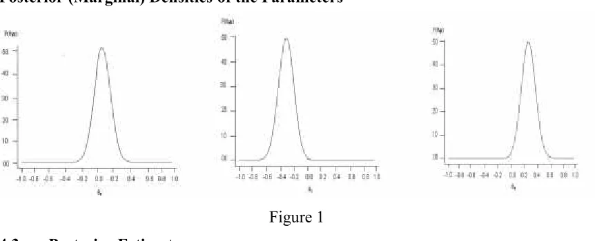
The graphical presentation of the marginal posterior distributions is given below.
Posterior (Marginal) Densities of the Parameters
Figure 1
4.3 Posterior Estimates
The posterior means and the joint modes of the parameters using the Jeffreys prior are considered as the posterior estimates of the parameters.
(a) Posterior Means: The posterior means for the parameters 1,2 and 3 using the
Quadrature method are obtained to be 0.05338, 0.31925 and 0.26192.
(b) Joint Posterior Modes: As the Jeffreys prior is not in closed form, so it is difficult to find the joint posterior modes mathematically so the posterior modes are obtained by sorting the maximum value of the densities. We observe that the densities are maximum at 0.0500,0.3250 and 0.2750 which are very close to the calculated values of the posterior means and hence the similar ranking of the treatments is observed.
4.4 Posterior Probabilities of the Hypotheses
Let us consider the hypotheses H12:12 vs H12:1 2
The posterior probability p12 ofH12isevaluated from the expression:
3
12 1 2 3 3
0
( ) ( , , )
p p p x d d d
, (8)The posterior probabilities are obtained by using quadrature method, we get the posterior probabilities as p12=0.98312 and q12 0.01688. We accept the hypothesis H12 that the
parameter θ1 is greater than the parameter θ2. Similarly we obtain p13 0.17064 with
13
q 0.82936, the decision is inconclusive for H13 and H13 but p23 0.0018769 and
23
q 0.998123 where H23is rejected and H23 is accepted with high probability.
4.5 Predictive Probabilities
The chance that treatment T1 is preferred to T2 in a single future comparison under the
TM model is computed in terms of predictive probability P(12) as
) 12 (
P =
(1 2) p(1,2)dθ1dθ2, (9)
where (12)is the preference probability of T1over T2 as defined in the model and
x
2 1,
(
p ) is the joint posterior distribution.
The predictive probabilities are obtained using quadrature method in SAS package. The value of the predictive probability P(12) is computed to be 0.64618. Similarly we get the
other predictive probabilities as P(13) 0.0048827 and P(23) 0.28155.
5. Appropriateness of the Tm Model
To test the hypotheses that the fit is good or appropriateness of the TM model for paired comparisons, we have the following hypotheses:
H0: The model is appropriate for any value of the parameter θ = θ0
H1: The model is not appropriate for any value of the parameter θ
where θ is the vector of parameters.
For testing the appropriateness of the model, we compared the observed and expected number of preferences. The expected number of preferences are calculated using the following expressions:
ij
n = rij {(i j)} and
ji
n = rij {(j i)} (10)
For this purpose, we use the usual2test with (m1)(m2)/2 degrees of freedom.
The observed and expected number of preferences are given in Table 2.
Table 2: The Observed and Expected Number of Preferences
Pairs(i,j) n12 n21 n13 n31 n23 n32
Obs. Freq. 18 12 14 16 07 23
The values of the different test-statistics are given below in Table 3.
Table 3: Goodness of Fit Tests
Test Name Test Statistics P-Value
Pearson 2 0.867000 0.352426
Anderson-Darling 0.323304 0.541112
Kolmogorov-Smirnov 0.227092 0.529792
Kuiper 0.454183 0.267540
Shapiro-Wilk 0.937117 0.636527
Hence from the above table, it is clear that there is no evidence that the model does not give good fit.
Comments and Conclusion
The Thurstone-Mosteller model is selected for a Bayesian analysis using the reference (Jeffreys) prior. The reference (Jeffreys) prior is derived for three treatment parameters. The prior has no closed form so it is used numerically by designing a program in SAS package. The posterior estimates (means and joint modes) of the parameters are determined. The posterior probabilities are evaluated for the Bayesian testing of hypotheses for comparing two parameters. The predictive probabilities are calculated for a single future comparisons of two treatments. The appropriateness of the model is also tested through different tests which indicate that the fit is good.
References
1. Abbas, N. and Aslam, M. (2009). Prioritizing treatments through paired comparison models, A Bayesian Approach.Pak. J. Stat., 25(1), 59-69.
2 Aslam, M. (2001). Bayesian analysis of the Rao-Kupper model using reference prior.Proc. Eighth stat. Sem. Karachi University, Pakistan.97-108.
3. Aslam, M. (2002). Bayesian analysis for paired comparison models allowing ties and not allowing ties.Pak. J. Stat., 25(1), 59-69., 18(1), 53-69.
4. Bradley, R. A. (1953). Some statistical methods in taste testing and quality evaluation.Biometrics,9, 22-38.
5. Bradley, R. A. (1976). Science, Statistics and paired comparisons. Biometrics, 32, 213-232.
6. Bradley, R. A., and Terry. M. E. (1952). Rank Analysis of Incomplete Block Design:І. The Method of Paired Comparisons.Biometrika,39, 324-345.
7. David, H. A. (1988). “The Method of Paired Comparisons,” second ed. Charles Griffin & Company Ltd., London.
9. Davidson, R. and Beaver, R. (1977). On extending the Bradley–Terry model to incorporate wi-pair order effects.Biometrics,33, 693–702.
10. Jeffreys, H. (1946). An invariant form for the prior probability in estimation problems.
11. Jeffreys, H. (1961).Theory of probability. Oxford, U.K. Claredon Press.
12. Johnson, R. A. and Ladalla. J. N. (1979). The large sample behavior of posterior distributions with sampling from multiparameter exponential family models and allied results.Sankhya,B, 41, 196-215.
13. McCullagh, P. (2000). Invariance and factorial models (RSS discussion paper, Oct 13 (1999) reply.J. Royal Statistical Society,62, 209–256.
14. Mosteller, F. (1951a), "Remarks on the Method of Paired Comparisons: I. The Least Squares Solution Assuming Equal Standard Deviations and Equal Correlations,"Psychometrika,16, 3-9.
15. Rao, P.V. and Kupper, L.L. (1967). Ties in paired-comparison experiments: a generalization of the Bradley–Terry model.Journal of American Statistical Association, 62, 194–204.
16. Stern, H. (1990). A continuum of paired comparison models. Biometrika, 77, 265-273.