On process capability and system availability analysis of the inverse Rayleigh distribution

On Process Capability and System Availability Analysis

of the Inverse Rayleigh Distribution

Sajid Ali

Department of Decision Sciences Bocconi University, Milan, Italy [email protected]

Muhammad Aslam

Department of Basic Sciences

Riphah International University, Islamabad, Pakistan [email protected]

Nasir Abbas

Department of Statistics

Government Postgraduate College Jhang, Pakistan [email protected]

Syed Mohsin Ali Kazmi

Sustainable Development Policy Institute (SDPI) Islamabad, 44000, Pakistan

[email protected]

Taha Hasan

Department of Statistics

Islamabad Model College for Boys, F-10/4, Islamabad, Pakistan [email protected]

Abstract

In this article, process capability and system availability analyses are discussed for the inverse Rayleigh lifetime distribution. Bayesian approach with a conjugate gamma distribution is adopted for the analysis. Different types of loss functions are considered to find Bayes estimates of the process capability and system availability. A simulation study is conducted for the comparison of different loss functions.

Keywords: Inverse Rayleigh Distribution; Loss Function; Process Capability; System Availability Analysis.

1. Introduction

increasing or decreasing failure rate depending upon the X 1.069543/  _or 1.069543/

X   .

In existing state of the art, Howlader et al. (2008) used the Bayesian approach for finding prediction bounds for Rayleigh and inverse Rayleigh lifetime models. Soliman et al. (2010) discussed Bayesian and classical estimation of the unknown parameter for the inverse Rayleigh distribution based on the lower record values. Rosaiah and Kantam (2010) discussed the acceptance sampling plan when the life test is truncated at a pre-assigned time for the inverse Rayleigh model. Dey (2012) studied the Bayes estimates of inverse Rayleigh distribution using squared error and LINEX loss functions while Aslam and Jun (2009) designed acceptance sampling plan from a truncated life test.

The rest of the article is organized as follows: The posterior distribution by considering gamma distribution as a prior is derived in Section 2. A simulation study for the parameter estimation under different loss functions, is also given in the same section. In Section 3, the process capability analysis for inverse Rayleigh distribution is discussed. The system availability analysis is given in Section 4. Finally, the last section has some concluding remarks and future proposals.

2. Posterior Distribution

The posterior distribution summarizes available probabilistic information on the parameter in the form of prior distribution and the sample information. The Bayes theorem is used to obtain a posterior distribution. Since the posterior distribution is an updated version of information, so the inference of posterior is challenging due to its complexity. In this section, we will use the inverse Rayleigh distribution as sampling distribution and combine it with the informative gamma prior. Let X X₁, ₂,...,X_n be a random sample taken from the inverse Rayleigh distribution. The probability distribution of inverse Rayleigh is:

 

2

exp , 0.

f x

x x

 _{ }

 _{ } 

 

The likelihood function of the inverse Rayleigh distribution with unknown parameter  is:

 

 

2 1 1

. 1 exp

n n

n

i

i

i i

L x

x

 

 

 

 _ _







From Eq. (1), one can easily observe that it looks similar to a gamma distribution. A conjugate prior can be easily constructed by replacing data with hyperparameters in Eq. (1). However, this conjugate will be gamma distribution. The gamma prior (GP) with hyperparameters 'a₁' and'b₁', has the following density:

 

   





1 1 1

1 1 1

1

exp , 0, 0, 0

a

b a

f b a b

a

    

    







 





1

1 1

2

1 1

2 1 1

1

1

| exp

a n

n

n

i i a n

i i

b x

p b

a n x

x

  



  



 



  _{ }

 

  _  _

  _{ }





So |x~Gamma





1

1 n

i i

b x









Remark

If we put a₁  b₁ 0in Eq. (2), then the posterior distribution for uniform prior can be

easily obtained. If a₁1,b₁0, we have the posterior distribution for Jeffreys' prior. Similarly, by using a₁ a₂ 2,b₁ 0.5, the expression for the chi-square prior can be obtained.

2.1. Bayes estimates under different Loss Functions

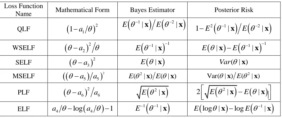
In this section, we consider different loss functions for the computation of Bayes estimate and posterior risk. In the usual Bayesian framework, the squared error loss function is commonly used. However, it does not reflect the reality because it gives equal weightage to over estimation and under estimation. For example, consider an example of dam construction where underestimation is forbidden, because if construction is underestimated then it will damage the nearby city. So to deal with such a situation, asymmetric instead of symmetric loss function is needed to consider. Therefore, for the analysis purpose, here we are comparing six loss functions given in the Table [1] (see Ali (2013), Ali et al. (2012) and references cited therein). Note that the general form of the first five loss functions can be written as:





( , ) ( , ) 1

L  a w a a 

where w( , ) a is a weight function.

Table 1: Bayes estimators and posterior risk under different loss functions

Loss Function

Name Mathematical Form Bayes Estimator Posterior Risk

QLF







 



1 2

| |

E  x E  x 2



 



1E  |x E  |x

WSELF

















SELF









MSELF

























 x x 

ELF a4 log









|

E  x









log | log |

2.2 Simulation study of the Bayes estimates (BE) and posterior risks (PR)

A simulation study is designed to see the effect of loss functions on the Bayes estimate. As in classical side the choice of an estimator is usually accomplished by using the minimum mean square error, therefore on Bayesian side, we are using posterior risk for the choice of Bayes estimator. A loss function which has a minimum posterior risk will be considered as the most suitable one for the further analysis related to process capability and system availability. The samples of different sizes for the selected value of , are generated from the inverse Rayleigh distribution using inverse transformation i.e. x  ln(u), where

u ~ [0,1]. Following hyperparametrs values are considered in the analysis:

1 1

3;a 9,b 4

   

1 1

20;a 171,b 9

   

1 1

25;a 145,b 6

   

For each selected sample size; 10,000 independent simulations were generated and average results are presented in the Tables [2-4].

Table 2: BEs and PRs for different loss functions when  3

n SELF QLF WSELF ELF PLF MSELF

25 2.7586

(0.22382) 2.5963 (0.03030) 2.6774 (0.08113) 2.6774 (0.02080) 2.7988 (0.08054) 2.839586 (0.028573)

50 2.8485

(0.13753) 2.7520 (0.01724) 2.8003 (0.04828) 2.8003 (0.01724) 2.8726 (0.04807) 2.896904 (0.016667)

100 2.9117

(0.07778) 2.8582 (0.00925) 2.8850 (0.02671) 2.8850 (0.00919) 2.9250 (0.02665) 2.938361 (0.009091)

500 2.9814

(0.1746) 2.9697 (0.00196) 2.9756 (0.00585) 2.9756 (0.00190) 2.9844 (0.00585) 2.987403 (0.001963)

1000 2.9897

(0.008858) 2.9837 (0.00099) 2.9867 (0.00296) 2.9867 (0.00098) 2.9911 (0.00296) 2.992501 (0.000990)

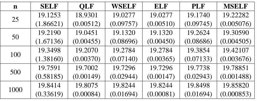
Table 3: BEs and PRs for different loss functions when  20

n SELF QLF WSELF ELF PLF MSELF

25 19.1253

(1.86621) 18.9301 (0.00512) 19.0277 (0.09757) 19.0277 (0.00510) 19.1740 (0.09745) 19.22282 (0.005076)

50 19.2190

(1.67136) 19.0451 (0.00455) 19.1320 (0.08696) 19.1320 (0.00450) 19.2624 (0.08686) 19.30590 (0.004505)

100 19.3498

(1.38160) 19.2070 (0.00370) 19.2784 (0.07140) 19.2784 (0.00365) 19.3854 (0.07133) 19.42107 (0.003676)

500 19.7591

(0.58185) 19.7002 (0.00149) 19.7296 (0.02944) 19.7296 (0.00147) 19.7738 (0.02943) 19.78851 (0.001488)

1000 19.8414

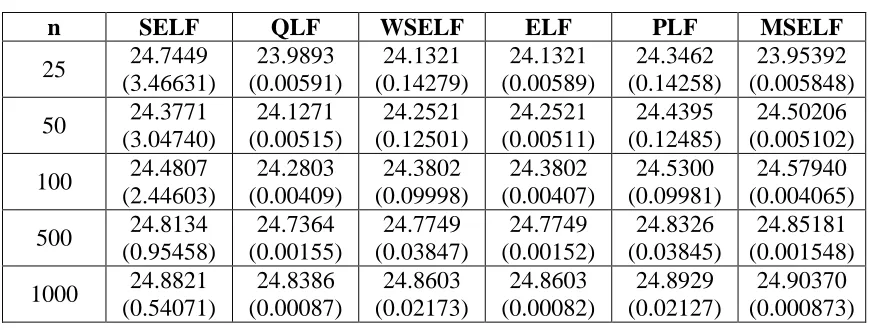
Table 4: BEs and PRs for different loss functions when  25

n SELF QLF WSELF ELF PLF MSELF

25 24.7449

(3.46631) 23.9893 (0.00591) 24.1321 (0.14279) 24.1321 (0.00589) 24.3462 (0.14258) 23.95392 (0.005848)

50 24.3771

(3.04740) 24.1271 (0.00515) 24.2521 (0.12501) 24.2521 (0.00511) 24.4395 (0.12485) 24.50206 (0.005102)

100 24.4807

(2.44603) 24.2803 (0.00409) 24.3802 (0.09998) 24.3802 (0.00407) 24.5300 (0.09981) 24.57940 (0.004065)

500 24.8134

(0.95458) 24.7364 (0.00155) 24.7749 (0.03847) 24.7749 (0.00152) 24.8326 (0.03845) 24.85181 (0.001548)

1000 24.8821

(0.54071) 24.8386 (0.00087) 24.8603 (0.02173) 24.8603 (0.00082) 24.8929 (0.02127) 24.90370 (0.000873)

From the Tables [2-4], it is clear that as the sample size increases, the Bayes estimate approaches to the nominal value of . The squared error loss function has the highest value of posterior risk as compared to other loss functions. On the base of posterior risk, we categorized the loss function as

ELFQLFMSELFPLFWSELF SELF

Using the data set given in Howlader et al. (2008), we have:

86

2 1

1

8.658513

i xi

 



 

 



1 9, 1 4

a  b  .

Table 5: Bayes estimates (BE) and posterior risks of a real data set under different loss functions

Loss

Function SELF QLF WSELF ELF PLF MSELF

BE 7.50483

(0.59286) 7.34683 (0.01052) 7.42583 (0.07899) 7.50483 (0.034210) 7.54422 (0.07879) 7.583817 (0.010417)

In case of a real data set, the relationship ELFQLFMSELFPLFWSELF SELF still holds. Therefore, we prefer the ELF, QLF and MSELF for the inverse Rayleigh distribution.

3. Process capability analysis of the inverse Rayleigh model

need to look for some suitable probability models to correctly capture the true process variations with reference to the characteristic(s) of interest.

There are different capability indices available in the quality control literature, which are used under different process scenarios, e.g. C_Np,C_Npk,C_Npm and C_Npmk Chen and Pearn (1997) and Tong and Chen (1988). For a recent comprehensive review on PCIs, one may see Yum and Kim (2011) and the references cited therein.

There are two main branches of Statistics namely Bayesian and Classical, and statistical methods to deal with practical situations, are generally developed under both approaches. Thus, the same is true about PCIs which are worked out in both, i.e. the Bayesian and classical setups, under normal and non-normal process distributions. Fan and Kao (2006) considered Taguchi capability index using Bayesian approach for estimation and testing concerns. Maiti et al. (2010) discussed about generalized process capability indices (GPCIs). Followed by Maiti and Saha (2012), this study is planned to investigate the GCPIs (cf. Maiti et al. (2010) and Maiti and Saha (2012)) from a Bayesian viewpoint under different symmetric and asymmetric loss functions for the inverse Rayleigh lifetime model.

Maiti et al. (2010) suggested a generalized measure defined as: C_py  p p₀, where p is the process yield (p=F(U)-F(L)), p0 is the desirable yield (p0=F(UDL)-F(LDL)), F(.) is the

cumulative distribution function , LDL and UDL the lower and upper desirable limits respectively. When the process is off center, then F(L)+F(U)1, and the index is defined

as C_pyk min(C_pyu,C_pyl)where

2

( ) ( )

0.5 pyu

F U F u

C   

 ₁

( ) ( )

0.5 pyl

F u F L

C   

 . Here uis the median (skewed distribution) of the distribution and the process center is to be located such that





( ) 0.5 ( ) ( )

F u_  F L F U ,  ₁ P X( LDL) and  ₂ P X( UDL). If the process target is T, then F T( )0.5F L( )F U( ) (known as symmetric tolerance), while if T0.5(L U ) _and





( ) 0.5 ( ) ( )

F T  F L F U (known as asymmetric tolerance). For such a situation, the index is

defined as:

2 1

( ) ( ) ( ) ( )

min ,

0.5 0.5

pTk

F U F T F T F L C

 

 



 

 

 

 .

The probability model for the inverse Rayleigh distribution is given as:

 

2

exp , 0

f x

x x

 _{ }

 _{ } 

  and its cumulative distribution function (cdf) is given by

2

( ) exp

F x

x





 

 _{ }

 .For theprocess which is modeled by the inverse Rayleigh distribution,

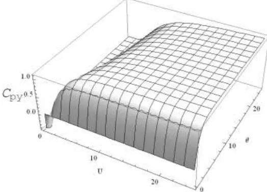
the generalized process capability index Cpy is given by:

0

0

2 2

exp exp

py

p C

p U L p

 

 _ _ _ _ _

   

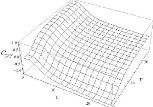
  . Figures [1-4] is the graphical presentation of

generalized capability index Cpy against  for varying choices of L and U. Note that in

Figure 1: Graphical Display of Cpy for Varying Choices of L and U (p0=0.9)

Figure 2: Graphical Display of Cpy for Varying Choices of L and U (p0=0.9,  3)

Figure 3: Graphical Display of Cpy for Varying Choices of L and U (p0=0.9,  20 )

20 40 60 80 100

0.2 0.4 0.6 0.8 1.0

Cpy

U 15 ,L 2 U 5,L 0.5 U 15 ,L 7 U 8,L 4 U 8,L 3 U 8,L 0

Figure 4: Graphical Display of Cpy for Varying Choices of L and U (p0=0.9, L=1)

To evaluate the Bayes estimate and respective posterior risk, we shall use SELF, PLF and MSELF loss functions. The reason to choose these three loss functions is: SELF is commonly used and accepted while PLF is asymmetric loss function and MSLF has posterior risk which is approximately equal to QLF (indicated from Tables [2-5]. To evaluate the Bayes estimate of Cpy under SELF, one needs to solve:

2 2

0 0 1

( _py | ) exp exp ( | )

E C p d

p U L

x    x 

 _{ }

 _ _ _ _ __

   

 



0

2 2

0

2

2 1

( _py | ) exp exp ( | )

E C p d

p U L

x    x 

 _{ }

 _ _ _ _ __

   

 



Therefore, the posterior risk will be *

 





( | ) ( | )

py py py

C E C x E C x

   . Similarly for other

loss functions, one can find the Bayes estimators and posterior risks. To see whether the inverse Rayleigh distribution is sensitive to either lower limit or upper limit, we used the net sensitivity analysis (cf. Maiti et al. (2010)). Net sensitivity analysis is defined as (p0)-1(f(U)-f(L)), where p0 is desirable yield in the proportion of nonconforming output,

F(UDL)+F(LDL)=1-. For the inverse Rayleigh distribution, the Table [6] contains the net sensitivity analysis.

Table 6: Net sensitivity analysis of the inverse Rayleigh distribution

p0=0.90 L=0.5,U=8,  =0.5

L=2,U=8,  =3

L=2,U=8,  =20

L=5,U=8,  =20

L=8,U=6,  =20

L=10,U=2,  =5

NS -1.20083 -0.381214 0.0260753 -0.0962531 0.054548 0.387354

will result in a small value of net sensitivity (in an absolute sense), which implies that distribution is less sensitive/robust with respect to L and U respectively. We noticed that if U<<L, distribution is more sensitive toward the upper specification limit. However, if L<U< then the distribution is sensitive to lower specification limit and the same is true about L<<U.

For simulation study, we considered different parameter values, i.e. 3, 20and 25 . For 3 we have PC nominal value 0.264084, 20 we have 0.692497 and for 25 we have PC value 0.683043. Note that these nominal values are calculated by assuming U=8 and L= 3. Table [7-9] presents the process capability indices under SELF, MSELF and PLF by using gamma prior. For large parameter’s value, we observed higher posterior risk which reduces with the increase of sample size. The Bayes estimates of process capability using SELF have smaller posterior risk value. This behavior is opposite to the Bayes

estimates given in Section 2 where we observed

ELFQLFMSELFPLFWSELF SELF . Thus, for the process capability index, the loss function can be categorized as SELFPLFMSELF.

Table 7: Bayes estimates and posterior risks of the process capability for  3

n SELF PLF MSELF

25 0.246447

(0.060736)

0.348529 (0.204163)

0.492895 (0.499998)

50 0.253081

(0.064050)

0.357911 (0.209659)

0.506163 (0.499999)

100 0.257698

(0.066408)

0.364440 (0.213483)

0.515396 (0.499998)

500 0.262745

(0.069035)

0.371578 (0.217665)

0.525491 (0.499999)

1000 0.263343

(0.069349)

0.372423 (0.218159)

0.526685 (0.4999997

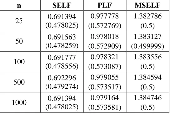
Table 8: Bayes estimates and posterior risks of the process capability for  20

n SELF PLF MSELF

25 0.691394

(0.478025)

0.977778 (0.572769)

1.382786 (0.5)

50 0.691563

(0.478259)

0.978018 (0.572909)

1.383127 (0.499999)

100 0.691777

(0.478556)

0.978321 (0.573087)

1.383556 (0.5)

500 0.692296

(0.479274)

0.979055 (0.573517)

1.384594 (0.5)

1000 0.691394

(0.478025)

0.979164 (0.573581)

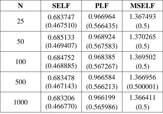
Table 9: Bayes estimates and posterior risks of the process capability for  25

N SELF PLF MSELF

25 0.683747

(0.467510)

0.966964 (0.566435)

1.367493 (0.5)

50 0.685133

(0.469407)

0.968924 (0.567583)

1.370265 (0.5)

100 0.684752

(0.468885)

0.968385 (0.567267)

1.369502 (0.5)

500 0.683478

(0.467143)

0.966584 (0.566213)

1.366956 (0.500001)

1000 0.683206

(0.466770)

0.966199 (0.565986)

1.366411 (0.5)

4. System availability analysis with the inverse Rayleigh distribution

Since the real world situations are dynamic, so the organizations in almost all parts of the world are becoming dependent on their systems. We (as a human) and companies heavily depend on different kinds of reliable systems. A system gives a performance until its failure is “available” before its failure. After the system failure, if we maintain them it will function again. Hence, the production of an item is available except for the period during which it is under repair. However, when the data on a complete system is not available, it is better to use the operational data about the system’s performance.

Availability of system has various meanings and different ways of its computation depending upon its use. It is defined as a percentage of the degree to which extent machinery and equipment is in an operable and a committable state at the point in time when it is needed. We can also declare it as a performance criterion for repairable systems that accounts for both the reliability and maintainability properties of a component or system. If somebody considers two kinds of information, i.e. the probability that the item will not fail (reliability) and the probability that the item is successfully restored after failure (maintainability); then an additional metric (availability) is needed for measuring the operational probability at the given time (cf. Khan and Islam (2012)).

Let the failure time X of each component be distributed as inverse Rayleigh with probability function:

 

2

exp , 0.

f x

x x

 _{ }

 _{ } 

  0  x .

where the mean time between failure (MTBF) is  . Also, let the repair time Y of each component is distributed as the inverse Rayleigh model with density:

 

2

exp , 0.

f y

y y

 _{ }

 _{ } 

  , 0  y .

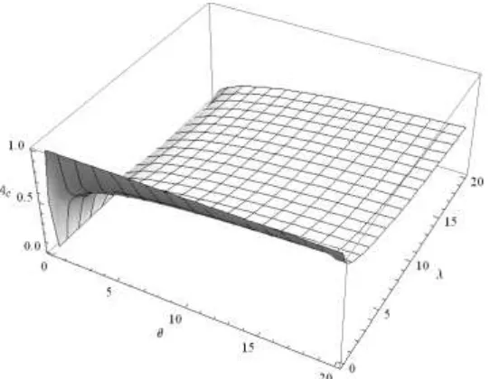
and the mean time to repair (MTTR) is . The steady state component availability, denoted by Ac, is the probability that the component is available in the long run and is given

asA MTBF

MTBF+MTTR +

c



 

  . If the system components are connected in a series, then

the availability of a series system is As = (Ac)m. The graphical presentation of system

availability is given in Figure [5], which is clearly an increasing function of the failure distribution’s parameter by keeping the small value of repair distribution’s parameter and vice versa.

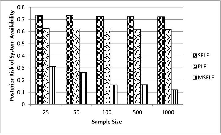
Figure 5: System availability of the inverse Rayleigh distribution

rapidly to a nominal value as compared to SELF and PLF. It is also worthy to mention that in case of system availability, the MSELF outperforms on the base of minimum posterior risk (cf. Figure [7]).

Figure 6: Bayes estimate comparison for the system availability analysis

Figure 7: Posterior risk comparison for the system availability analysis

5. Conclusion

In this article, the process capability and system availability analysis of the inverse Rayleigh distribution is given. We used the Bayesian method for the unknown parameter estimation. Different types of loss functions are also used for the Bayesian estimation. A

0.6 0.605 0.61 0.615 0.62 0.625 0.63

25 50 100 500 1000

B

ay

e

s E

sti

m

ate

S

yste

m

A

vai

lab

ili

ty

Sample Size

SELF

PLF

MSELF

0 0.1 0.2 0.3 0.4 0.5 0.6 0.7 0.8

25 50 100 500 1000

Post

e

ri

o

r R

isk

o

f Sy

ste

m

A

vai

lab

ili

ty

Sample Size

SELF

PLF

detailed simulation study using different sample sizes is given in this article. It is observed that the posterior risks of the estimates of the parameters are large for the larger values of the parameters and vice versa. However, the posterior risk of parameters is reduced as the sample size increases. In case of Bayes estimates, we categorized the loss function as ELFQLFMSELFPLFWSELF SELF by using posterior risk as a comparative measure. However, in case of process capability analysis, the ordering of loss function is SELFPLFMSELFand vice versa for system availability analysis. We considered SELF, PLF and MSELF in case of system availability and process capability analysis; because SELF is widely used and accepted, PLF is an asymmetric loss function while WSELF has a minimum posterior risk for the Bayes estimates (discussed in Section 2). In future, this work can be extended using inverse Rayleigh truncated distribution.

Acknowledgement

The authors would like to thank the referees for their careful reading of the paper and constructive remarks, which lead to a better and clear presentation of the article.

References

1. Ali, S. (2015). On the Bayesian estimation of weighted Lindley Distribution. Journal of Statistical Computation and Simulation, 85 (5), 855-880.

2. Ali, S., Aslam, M., Kazmi, S. M. A. and Abbas, N. (2012). Scale parameter estimation of the Laplace model using different asymmetric loss functions, International Journal of Statistics and Probability, 1 (1), 105-127.

3. Aslam, M. and Jun, Chi-Hyuck, (2009). A group acceptance sampling plans for truncated life tests based on the inverse Rayleigh and Log-Logistic distributions, Pakistan Journal of Statistics, 25(2), 107-119.

4. Chen, K. S., and Pearn, W. L. (1997). Capability indices for non-normal distributions with an application in electrolytic capacitor manufacturing. Microelectronics and Reliability, 37, 1853-1858.

5. Dey, S. (2012). Bayesian estimation of the parameter and reliability function of an inverse Rayleigh distribution, Malaysian Journal of Mathematical Sciences, 6(1), 113-124.

6. Fan, S, S. and Kao, C. (2006). Development of confidence interval and hypothesis testing for Taguchi capability index using a Bayesian approach. International Journal of Operations Research, 3 (1), 56-75.

7. Howlader, H. A., Hossain, M. A. and Makhnin, O. (2008). Bayesian prediction bounds for Rayleigh and inverse Rayleigh lifetime models, Journal of Applied Statistical Science, 17 (1), 131-142.

9. Maiti, S. S., Saha, M. and Nanda, A. K., (2010). On generalizing process capability indices, Journal of Quality Technology and Quantitative Management, 7 (3), 279– 300.

10. Maiti, S. S. and Saha, M. (2012). Bayesian estimation of generalized process capability indices, Journal of Probability and Statistics, Volume 2012, Article ID 819730, 15 pages, doi:10.1155/2012/819730.

11. Rosaiah, K. and Kantam, R. R. L. (2010). Acceptance sampling based on the inverse Rayleigh distribution, Economic Quality Control, 20 (2), 277-286.

12. Soliman, A. A. and Al- Aboud, F. M. (2008). Bayesian inference using record values from Rayleigh model with application, European Journal of Operational Research, 185 (2), 659-672.

13. Soliman, A., Amin, E. A. and Abd-El Aziz, A. A. (2010). Estimation and prediction from inverse Rayleigh distribution based on lower record values, Applied Mathematical Sciences, 4 (62), 3057 – 3066.

14. Tong, L.I., and Chen, J.P. (1998). Lower confidence limits of process capability indices for non-normal process distributions, International Journal of Quality and Reliability Management, 15(8/9), 907-919.