S O F T W A R E
Open Access
DPASF: a flink library for streaming data
preprocessing
Alejandro Alcalde-Barros
*, Diego García-Gil
*, Salvador García and Francisco Herrera
*Correspondence: [email protected]; [email protected]
Department of Computer Science and Artificial Intelligence, CITIC-UGR (Research Center on Information and Communications Technology), University of Granada, Calle Periodista Daniel Saucedo Aranda, 18071 Granada, Spain
Abstract
Background: Data preprocessing techniques are devoted to correcting or alleviating errors in data. Discretization and feature selection are two of the most extended data preprocessing techniques. Although we can find many proposals for static Big Data preprocessing, there is little research devoted to the continuous Big Data problem. Apache Flink is a recent and novel Big Data framework, following the MapReduce paradigm, focused on distributed stream and batch data processing.
In this paper, we propose a data stream library for Big Data preprocessing, named DPASF, under Apache Flink. The library is composed of six of the most popular and widely used data preprocessing algorithms. It contains three algorithms for discretization, and three algorithms for performing feature selection.
Results: The algorithms have been tested using two Big Data datasets. Experimental results show that preprocessing can not only reduce the size of the data, but also maintain or even improve the original accuracy in a short period of time.
Conclusion: DPASF contains algorithms that are useful when dealing with Big Data data streams. The preprocessing algorithms included in the library are able to tackle Big Datasets efficiently and to correct imperfections in the data.
Keywords: Flink, Big data, Machine learning, Data preprocessing
Background
In recent years, the amount of data generated can no longer be treated directly by humans or manual applications, there is a need to analyze this data automatically and on a large scale [1]. This is what is know to be Big Data, data generated at high volume, velocity and variety. This kind of data requires a new high-performance processing and it can currently be found in many different fields [2].
In order to extract quality information from data, a previous step to learning must be performed. This is known as data preprocessing [3], this step is almost mandatory in order to obtain a good model. Data preprocessing [4] deals with missing values, noise, and redundant features [1,5] among other factors.
Data streams [6] are sequences of unbounded and ordered data that arrive one at a time. This imposes restrictions on the learning algorithms which do not appear in static data. Therefore, new algorithms that can deal with this kind of data must be developed.
To address the problem of dealing with such a large amount of data in the Big Data era, distributed frameworks such as Apache Spark [7] and Apache Flink [8,9] have been developed. Apache Spark is well known and designed to be a fast and general engine for large-scale in-memory data processing. Apache Flink focuses, on the other hand, on distributed streams and batch data processing [10]. Flink is also the only system to incor-porate a distributed dataflow runtime that exploits streaming pipelined executions for both stream and batch data processing. It also provides a fault tolerance mechanism, using a lightweight checkpoint system, which ensures that every data example will be reflected exactly once [11].
This paper presents the data stream library for Big Data preprocessing named DPASF, where six data preprocessing algorithms are implemented for Apache Flink, focusing on the discretization and feature selection problems. The algorithms chosen are those that have obtained the best performance in the survey carried out in [6]. In this sur-vey authors summarize, categorize and analyze the most relevant contributions on data preprocessing that cope with streaming data. The selected algorithms are InfoGain [12], FCBF [13] and OFS [14] for feature selection and IDA [15], LOFD [16] and PiD [17] for discretization.
The rest of the paper describes the theoretical background of the algorithms, experi-mental results and a brief tutorial on how to use them. Source code is available on GitHub1 [18]. The algorithms chosen are the most representative in data streaming preprocessing and, in addition, have shown positive results.
Big Data
In general, Big Data [19–22] is known to be data that is too big or too complex to handle with conventional tools and with a single machine. For this reason, there is an increas-ing need to develop new tools that can handle all this amount of data efficiently. As a result, distributed frameworks like Hadoop [23], Spark [7] and Flink [8] were developed. These types of frameworks allow large amounts of data to be processed in a scalable way.
One common way to define Big Data is to describe it in terms of three dimensions, also known as the 3 V’s [24] (Volume, Velocity and Variety). Volume just refers to how much data there is. Velocity refers to the speed at which data is processed and analyzed. Lastly, Variety refers to how many different data formats there are to be analyzed.
Data Streaming
The main characteristics of streaming data [25] are the following. In streaming data, instances are not available beforehand, they become available in a sequence fashion, one by one, or in batches. Instances can arrive quickly and at irregular time intervals. As streaming data is unbounded, it may be infinite and therefore cannot be stored in mem-ory. Each instance is accessed usually only once and is then discarded. In order to provide real-time processing, instances are processed within a limited amount of time. The intrin-sic characteristics of data are subject to change over time, this is what is know as concept drift [26].
Data Preprocessing
Before applying any data mining process, it is necessary to adapt the data to the requirements imposed by each learning algorithm and clean the data properly.
Although data preprocessing is a critical step, it is often time consuming. There are two types of data preprocessing, those designed to reduce the complexity in the data, and those designed to prepare the data, this means data transformation, cleaning, normal-izing etc. The former is called data reduction, the latter data preparation. When these techniques are applied, the data is in its final stage to be fed to the data mining algorithm. Among data transformation, feature selection [1,27] takes care of selecting only rele-vant and non-redundant attributes. The aim of this type of data preprocessing is to obtain a subset of the original data that stills maintains the ability to describe the inherent con-cept. As a side effect, reducing the complexity of the data also results in better efficiency in terms of the amounts of time to learn a model, as well as preventing over-fitting.
Discretization [15] is a technique that reduces the complexity of the data by dividing the domain of the variables into bins defined by cut points. This process transforms quan-titative values into qualitative, as cut points define a set of non-overlapping intervals. Once the algorithm has computed cut points for each attribute, data is then mapped to its corresponding interval [1].
Apache Flink
Although Apache Spark and Apache Flink may appear to be similar, they are designed to address different problems. Apache Spark process all data using a batch approach, it lacks a true stream processing. Apache Flink fills this gap. Flink provides both kinds of processing, batch and streaming, except Flink process streaming data as it happens, in an online fashion. In other words, Spark "emulates" streaming by processing streaming data in mini-batches, whereas Flink process them online. This makes Flink more efficient in terms of low latency.
Apache Flink has a fault tolerance system in order to recover from exceptions that may occur. It is designed to work at low latency even with large amounts of data.
Theoretical description of the algorithms presented
This section presents a theoretical description of the implemented algorithms, as well as an introduction to feature selection (InfoGain [12], FCBF [13] and OFS [14]) and discretization (IDA [15], LOFD [16] and PiD [17]).
Feature Selection
Feature selection [28] is meant to reduce the dimensionality of a dataset by removing irrelevant and redundant features. By doing this, a subset of the original features that still describes the inherent concept behind the data is returned. FS methods can be divided in the following categories:
• Wrapper Methods It uses an external evaluator, which depends on a learning
algorithm.
• Filtering Methods It uses selection techniques based on separability measures or statistical dependencies.
• Embedded Methods It uses a search procedure implicitly embedded in the classifier
In general, filtering methods tend to achieve better results when generalizing due to learning independence. In addition, filter methods are more efficient than wrapper meth-ods, since the latter need to learn a model first. Therefore, in the context of big data, filtering methods are more widely used. Information Gain [12], OFS [14] and FCBF [13] are the most popular preprocessing algorithms in this area.
Information Gain
This feature selection scheme, described in [12] is composed of two steps: An incremental feature ranking method, and an incremental learning algorithm that can consider a subset of the features during prediction.
For this algorithm, the conditional entropy with respect to the class is computed with
H(X|Y)= −
j
P(yj)
i
P(xi|yj)log2(P(xi|yj)) (1)
then, the Information Gain (IG) is computed for each attribute with
IG(X|Y)=H(X)−H(X|Y) (2)
Once the algorithm has all Information Gain values for each attribute, the topN are selected as best features.
Online Feature Selection (OFS)
OFS [14] proposes an -greedy online feature selection method based on weights generated by an online classifier (neural networks) which makes a trade-off between exploration and exploitation of features.
The main idea behind this algorithm is that when a vectorxfalls withing aL1 ball, most of its numerical values are concentrated in its largest elements, therefore, removing the smallest values will result in a small change in the original vectorxas measured by theLq
norm. This way, the classifier is restricted to aL1 ball:
R=
w∈Rd:||w||1≤R
(3)
OFS maintains an online classifier wt with at mostB nonzero elements. When an
instance(xt,yt)is incorrectly classified, the classifier gets updated through online
gra-dient descent and then it is projected to aL2 ball to delimit the classifier norm. If the resulting classifierwˆt+1has more thanBnonzero elements, the elements with the largest
absolute value will be kept inwˆt+1.
The above approach presents an inefficiency, even although the classifier consists ofB nonzero elements, full knowledge of the instances is required, that is, each attributext
must be measured and computed. As a solution, OFS limit online feature selection to no more thanBattributes ofxt
Fast Correlation-Based Filter (FCBF)
The algorithm chooses as a correlation measure the entropy of a variableX, which is defined as
H(X)= −
i
P(xi)logP(xi) (4)
and the entropy ofXafter observing values of another variableYis defined as
H(X|Y)= −
j
P(yj)
i
P(xi|yj)log2(P(xi|yj)) (5)
whereP(xi)is the prior probability for all values ofXandP(xi|yj)is the posterior
prob-ability ofXgiven the values ofY. With this information, a measure calledInformation Gaincan be defined:
IG(X|Y)=H(X)−H(X|Y) (6)
According to IG, a featureY is more correlated toXthan to a featureZ ifIG(X|Y) > IG(Z|Y).
Now we are ready to define the main measure for FCBF,symmetrical uncertainty[29]. As a pre-requisite, data must be normalized in order to be comparable.
SU(X,Y)=2
IG(X|Y) H(X)+H(Y)
(7)
SUcompensate the bias inIGtoward features with more values and normalizes its values to the range [ 0, 1]. ASUvalue of 1 indicates total correlation whereas a value of 0 indicates independence.
The algorithm follows a two step approach, first, it has to decide if a feature isrelevant to the class and two, decide if those features areredundantwith respect to each other.
To solve the first step, a user definedSU threshold can be defined. IfSUi,cis theSU
value for featureFiwith the classc, the subsetSof relevant features can be defined with
a thresholdδsuch that∀Fi∈S, 1≤i≤N,SUi,c≥δ.
For the second step, in order to avoid analysis of pairwise correlations between all fea-tures, a method to decide whether the level of correlation between two features inSis high enough to produce redundancy is needed in order to remove one of them. Examin-ing the valueSUj,i∀Fj ∈ S(j= i)allows the level to whichFjis correlated by the rest of
features inSto be estimated.
The last piece of the algorithm comprises two definitions:
Definition 1(Predominant Correlation). The correlation between a feature Fiand the
class C is predominant iff SUi,c≥δand∀Fj∈S(j=i)Fjsuch that SUj,i≥SUi,c
If such feature Fjexists for a feature Fi, it is called a redundant peer of Fiand it is added
to a set SPiidentifying all the redundant peers for Fi. SPiis divided into two parts: S +
Piand
S−Pi, where SP+i= {Fj|Fj∈SPi,SUj,c>SUi,c}and S−Pi= {Fj|Fj∈SPi,SUj,c≤SUi,c}
Definition 2(Predominant Feature). A feature is predominant to the class if its cor-relation to the class is predominant or can become predominant after removing all its redundant peers.
Heuristic 1(whenS+Pi = ∅).Fiis a predominant feature, delete all features inSP−iand
stop searching for redundant peers for those features.
Heuristic 2(whenS+Pi= ∅). All features inSP+iare processed before making decisions in Fi. If none of them become predominant go to Heuristic 1, or else removeFiand decide
if features inSP−
ineed to be removed based on other features inS .
Heuristic 3(Start point). The algorithm begins examining the feature with the largest SUi,c, as this feature is always predominant and acts as a starting point for the removal of
redundant features.
Discretization
Broadly speaking, discretization [30] translates quantitative data into qualitative data, trying to avoid an overlap between the continuous domain of the variable. This process results in a mapping of a value to a given interval. For this reason, discretization can be considered as a data reduction process, since it reduces data from a numerical domain to a subset of categorical values.
More formally, a discretizationδof a numeric attributeXiis a set ofmintervals called
bins. The bins are defined by cut points{k1,. . .,km−1}that divide the domain ofXiintom
bins whereb1=[−∞,k1] ,bm=[km−1,∞] and for 1<i<m,bi =(ki−1,ki]. Therefore,
a discretization for an attributeXiis a mapping between valuesvofXiand its bin indexes
δv=zsuch thatv∈bz.
The most popular discretization algorithms are IDA [15], PiD [17] and LOFD [16].
Incremental Discretization Algorithm (IDA)
IDA [15] approximates quantile-based discretization on the entire data stream encoun-tered to date by maintaining a random sample of the data which is used to calculate the cut points. IDA uses the reservoir sampling algorithm to maintain a sample drawn uniformly at random from the entire stream up until the current time.
In IDA, a random sample is used because it’s not feasible for high-throughput streams to maintain a complete record of all the values seen so far. The sample method used is called reservoir sampling [31], and mantains a random sample ofsvaluesVifor each attribute
Xi. The firstsvalues that arrive for eachXiare added to its correspondingVi. Thereafter,
every time a new instancexn,yn
arrives, each of its valuesxinreplace a randomly selected value of the correspondingViwith probabilitys/n.
Each value of each attribute is stored in a vector of interval heaps [32].Vij stores the values for the jth bin ofX
i. The reason to use a Interval Heap is that it provides
effi-cient access to minimum and maximum values in the heap and direct access to random elements within the heap.
Partition Incremental Discretization algorithm (PiD)
PiD [17] performs incremental discretization. The basic idea is to perform the task in two layers. The first layer receives the sequence of input data and keeps some statistics on the data using many more intervals than required. Based on the statistics stored by the first layer, the second layer creates the final discretization. The proposed architecture processes streaming examples in a single scan, in constant time and space even for infinite sequences of examples.
The first layer receives the sequence of input data and the range of the variable and keeps some statistics on the data using many more intervals than required. The range of the variable is used to initialize the cut points with the same width. Each time a new value arrives, this layer is updated in order to compute the corresponding interval for the value. Each interval has a internal count of the values it has seen so far. When a counter for an interval reach a threshold, a split process is triggered to generate two new intervals. If the interval triggering the split process is the last or the first, a new interval with the same step is created. Otherwise the interval is split in two. In summary, the first layer simplifies and summarizes the data.
Based on the statistics stored by the first layer, the second layer creates the final dis-cretization. The proposed architecture processes streaming examples in a single scan, in constant time and space even for infinite sequences of examples. To do so, this layer merges the set of intervals computed in the previous layer.
PiD stores the information about the number of examples per class in each interval in a matrix. In this matrix, columns correspond with the number of intervals and rows with the number of classes. With this information, the conditional probability of an attribute belonging to an interval given that the corresponding example belongs to a class can be computed asP(bi<x≤bi+1|Classj).
To perform the actual discretizationRecursive entropy discretization[33] is used. This algorithm was developed by Fayyad and Irani [34]. It uses the class information entropy of two candidate partitions to select the boundaries for discretization. It begins search-ing for a ssearch-ingle threshold that minimizes the entropy over all possible cut points, then, it is applied recursively to both partitions. It uses theminimum description length[35] principle as stop criteria. The algorithm works as follows:
First, the entropy before and after the split is computed as well as its information gain. Then, the entropy for both left and right splits is computed and finally the algorithm checks if the split is accepted using the following formula
Gain(A,T;S) <log2(N−1)
N +
(A,T;S)
N (8)
whereNis the number of instances in the setS,
Gain(A,T;S)=H(S)−H(A,T;S) (9)
and
(A,T;S)=log2 3k−2
−[k·H(S)−k1·H(S1)−k2·H(S2)] (10)
where kiis the number of class labels represented in the set Si.
Local Online Fusion Discretizer (LOFD)
The algorithm is composed of two phases, the main process, at instance level, and the merge/split process, at interval level. The main process works as follows. First, discrete interval are initialized following the static process defined in [36]. The discretization is then performed on the firstinitThinstances. From that moment on, LOFD updates the scheme of intervals in each iteration and for each attribute. For each new instance, it retrieves its ceiling interval (implemented as a red-black tree). If the point is above the upper limit a new interval is generated at that point, making that point the new maximum for the current attribute. A merge between the old and the new last interval is evaluated by computing the quadratic entropy, if the result is lower than the sum of both parts, the merge is accepted.
Finally, each point is added to a queue with a timestamp to control future removals in case the histogram overflows. If necessary, LOFD recovers points from the queue in ascending order and removes them until there is space left in the histogram.
The split/merge phase is triggered each time a boundary point is processed. The new boundary point splits an interval in two, one interval contains the points in the histogram with values less than or equal to the new point and keeps the same label. Each time a new interval is generated, the merge process is triggered for the intervals being divided and their neighbors.
Implementation
This section presents the distributed design of the six implemented algorithms. For the implementation of the methods, we have used some basic Flink primitives. Here we outline those that are more relevant for the algorithms:
• mapThe Map transformation applies a user-defined map function to each element
of a DataSet
• reduceA Reduce transformation reduces the dataset to a single element using a user-defined reduce function.
• mapPartitionMapPartition transforms a parallel partition in a single function call. • reduceGroupA GroupReduce transformation that is applied to a grouped DataSet calls a user-defined group-reduce function for each group. The difference between this and Reduce is that the user defined function gets the whole group at once.
Algorithm 1 shows pseudocode for FCBF, the SU value is computed for each attribute in parallel. All SU values are then filtered according to the threshold param-eter and then sorted in descending order. With these final sorted values, the FCBF algorithm is applied as originally described in [13]. Algorithm 2 shows how Sym-metrical Uncertainty is computed in a distributed fashion. First, each parallel parti-tion computes the partial counts of each value, then this partial counts are aggre-gated using a reduce function in order to compute the total counts. With this information, probabilities for each value are computed and the entropy and mutual information are calculated. Finally, it returns the corresponding SU value for that attribute.
Algorithm 1FCBF Algorithm
1: Input:dataa DataSet LabeledVector (label, features) 2: Input:thrthreshold
3: Output:DataSet with the most important features 4: su←
5: fori←0 untilnAttrsdo
6: attr←
7: mapinstance∈data
8: (label,featurei)
9: end map
10: yieldSU(attr)
11: end for
12: suSorted←FILTER(su > thr).SORTDESC
13: sBest←FCBF(suSorted)
14: returnsBest
attribute its computed and stored in gains. Algorithm 4 shows how frequencies are computed.
Algorithm 5 shows the pseudocode for OFS [14], this algorithm maps each label and feature with their corresponding value for the original OFS algorithm.
Algorithm 6 shows pseudocode for IDA [15]. This algorithm first computes the cut points for the dataset with the desired number of bins. In order to compute the cut points, each instance is mapped to the result of IDA, which returns the computed cut points. To do so, each feature is zipped with its index, and then folded with its corresponding class label and a zero feature vector that will be filled in each iteration of the fold operation, with
Algorithm 2Symmetrical Uncertainty function (SU)
1: Input:attrAttribute to comute SU to 2: Output:SU value forattr
3: xypartialCounts← 4: mapPartition(y,x)∈attr
5: xPartialCounts←COMPUTECOUN TS(x)
6: yPartialCounts←COMPUTECOUN TS(y)
7: (xPartialCounts,yPartialCounts) 8: end mapPartition
9: totalCounts←REDUCE(xypartialCounts)
10: su←
11: map(xcounts,ycounts,x,y)∈totalCounts
12: px←PROB(x)
13: py←PROB(y)
14: hx←EN TROPY(x)
15: hy←EN TROPY(y)
16: mu←MUTUALINFORMATION(x,y)
Algorithm 3InfoGain Algorithm
1: Input:dataa DataSet LabeledVector (label, features) 2: Input:selectNFNumber of features to select
3: Output:DataSet with the mostselectNFimportant features 4: freqs←FREQUENCIES(data, groupBy label)
5: H←EN TROPY(freqs)
6: gains←
7: mapi∈0 untilnFeatures
8: freqs←FREQUENCIES(data,featurei)
9: px←PROBS(freqs)
10: H←EN TROPY(freqs)
11: H(Y|Featurei)←CONDITIONALEN TROPY(freqs)
12: H−H(Y|Featurei)
13: end map
14: returnSELECTFEATURES(selectNF, gains)
Algorithm 4Frequencies function
1: Input:attrattribute to compute frequencies to
2: Input:f function to group by
3: Output:Frequencies forattrusingf
4: grouped←groupBy(data,f)
5: freqs←reduceGroup(grouped) 6: returnfreqs
the returned value of the IDA algorithm. Once cut points are stored, line 5 in Algorithm 6 discretizes the data according to those cut points.
Algorithm 7 shows pseudocode for PiD [17], this algorithm first initializes the required data structures using a map function, this map function expands the dataset and adds it to a histogram and a count of the total number of instances seen so far. Then this data is reduced, computing in each reduce step the layers one and two as described in the original
Algorithm 5OFS Algorithm
1: Input:dataa DataSet LabeledVector (label, features)
2: Input:ηparameter
3: Input:λparameter
4: Input:selectNFNumber of features to select
5: Output:DataSet with the mostselectNFimportant features 6: finalweights←
7: map(label,features)∈data
Algorithm 6IDA Algorithm
1: Input:dataa DataSet LabeledVector (label, features) 2: Input:binsnumber of bins
3: Output:Discretized dataset with desired number ofbins 4: cuts←
5: map((y,x)∈data)
6: zipped←ZIPWITHINDEX(x)
7: FoldLeft((y,emptyfeature))(IDA()) 8: end map
9: returnDISCRETIZE(data, cuts)
algorithm [17]. Once this reduce stage has been completed, it returns the discretized data using the previously computed cut points.
Algorithm 8 shows pseudocode for LOFD [16]. This algorithm first instantiates a LOFD helper, and maps the data according to the computed cut points this helper returns. Once all cutpoints have been collected, the reduce function extracts only the most recently computed cut points and applies discretization based on those same cut points.
Results
This section presents in detail the six algorithms implemented in Apache Flink, there are three algorithms for feature selection and three for discretization.
Examples
The software has been implemented in the Scala programming language2. As mentioned above, DPASF consists of six algorithms for data streams, three discretization methods and three feature selection methods. The software can be found on GitHub3. The next section presents how to use each algorithm in Apache Flink.
Algorithm 7PiD Algorithm
1: Input:dataa DataSet LabeledVector (label, features) 2: Input:αparameter
3: Input:stepparameter
4: Output:Discretized dataset
5: cuts←
6: mapinstance∈data
7: (instance,Histogram, 1) 8: end map
9: reduce(m1,m2)∈cuts 10: UPDATELAYER1(m1, m2)
11: UPDATELAYER2(m1, m2)
12: end reduce
Algorithm 8LOFD Algorithm
1: Input:dataa DataSet LabeledVector (label, features) 2: Output:Discretized dataset
3: lofd←LOFDInstance 4: cuts←
5: mapx∈data
6: discretized←lofd.applyDiscretization(x)
7: fors in 0 until discretized.sizedo 8: lofd.getCutpoints(s)
9: end for
10: end map
11: reduce(_,b)∈cuts
12: b
13: end reduce
14: returnDISCRETIZE(data, cuts)
Usage
Feature Selection
FCBF In order to benefit from the Apache Flink framework, symmetrical uncertainty computations for each pair of attributes are distributed across each node in order to speed up the process.
Suppose the data set to be used is the Abalone DataSet4, load it into Apache Flink:
Then, aFCBFTransformermust be instantiated, configure its parameters and finally define a pipeline:
After fitting the algorithm, callingtransformonfcbfwill return the Abalone data set with the most important features.
The use ofInfoGainTransformeris similar:
OFS One difference of OFS with respect to the previous algorithms is that it does not require a fitting phase:
Discretization
In this section the usage of the discretization methods is presented. The Iris5DataSet was used, loaded as:
IDA For IDA, cut points are computed in parallel, in order to get the most recent computed cut point, data is reduced to get the latest set of cuts.
Table 1Information about DataSets for experiments
DataSet Instances Attributes Classes
ht_sensor 929000 11 3
skin_nonskin 245000 3 2
In PiD, data must be normalized in the previous step, so aChainTransformeris used in the pipeline.
LOFD For LOFD, a PiD-like approach is used. First, all features are mapped in order to extract the necessary information from them, then, data is reduced to extract the final cut points to perform discretization.
Results
The experimental set up has used two datasets, ht_sensor andskin_nonskin, and are described in Table1.
All algorithms have been tested with KNN and Decision Trees using 5-fold cross vali-dation. A baseline is fitted without any preprocessing steps, and another is fitted with the corresponding preprocessing algorithm. In addiction KNN has been fitted with k = 3 and k = 5.
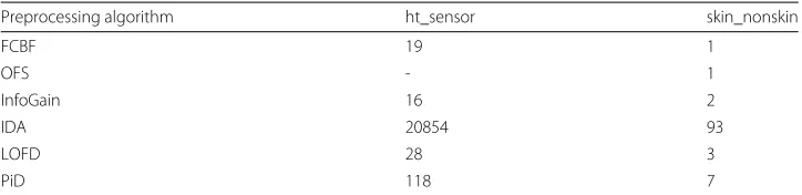
All the feature selection methods have been set up to select 50% of the features. Table2shows the amount of time it took to preprocess the data. The worst algorithm by far is IDA, which took about 5 h to finish for ht_sensor. On the contrary, the fastest was InfoGain. OFS could not be measured as it only accepts binary datasets. It is worth mentioning that these experiments could not have been possible in normal environments due to the amount of time they would have taken.
Table 2Times in seconds
Preprocessing algorithm ht_sensor skin_nonskin
FCBF 19 1
OFS - 1
InfoGain 16 2
IDA 20854 93
LOFD 28 3
Table 3Accuracy for KNN with k = 3
k = 3 ht_sensor skin_nonskin
Baseline 0.9998 0.9995
FCBF 0.8965 0.8642
OFS - 0.8985
InfoGain 0.9999 0.9825
IDA 0.8845 0.6591
LOFD 0.9662 0.9755
PiD 0.9999 0.9966
The best results are in bold
For all experiments we have used a cluster composed of 14 computing nodes. The nodes hold the following characteristics: 2 x Intel Core i7-4930K, 6 cores each, 3.40 GHz, 12 MB cache, 4 TB HDD, 64 GB RAM. Regarding software, we have used the follow-ing configuration: Apache Flink 1.6.0, 238 TaskManagers (17 TaskManagers/core), 49 GB RAM/node.
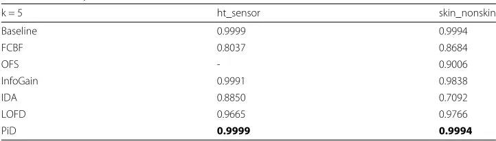
Tables 3 and 4 show the accuracy obtained by the algoritms, as well as the accu-racy without any preprocessing. The three feature selection methods obtain considerable results, even when they are configured to remove half the features on the datasets. FCBF is not among the best, but it is among the fastest. This may be due to the fact that it avoids computing pairwise comparisons when selecting features. Also, FCBF can not be set to select a fixed number of features, it uses a threshold to select features based on its SU value, so in some cases it will select less than half the features. InfoGain also gives excel-lent results, close to the baseline and even improves when k=3. Among the discretizers, PiD outperforms baseline in all cases except for skin-nonskin with k=3.
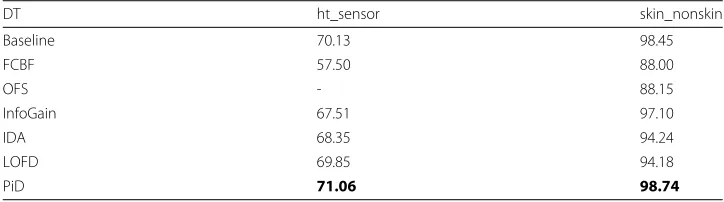
Table5shows accuracy for a Decision Tree model, results are consistent with the previ-ous model. In general, feature selection methods result in a decrease in accuracy whereas discretization methods are consistent with baseline, albeit PiD improves accuracy.
Conclusions
In this paper we have tackled the Big Data stream preprocessing problem. We have cre-ated a library for Big Data data stream preprocessing called DPASF that is implemented in the Big Data streaming framework Apache Flink. This library includes six popular data preprocessing algorithms. Three of the algorithms are focused on discretization, while the other three are focused on feature selection tasks. All the algorithms have been redesigned for the map reduce framework so they can cope with Big Data datasets.
The performance of the six algorithms in Big Data scenarios has been analyzed using two Big Data datasets. Experimental results have shown that preprocessing can improve
Table 4Accuracy for KNN with k = 5
k = 5 ht_sensor skin_nonskin
Baseline 0.9999 0.9994
FCBF 0.8037 0.8684
OFS - 0.9006
InfoGain 0.9991 0.9838
IDA 0.8850 0.7092
LOFD 0.9665 0.9766
PiD 0.9999 0.9994
Table 5Accuracy for Decision Trees
DT ht_sensor skin_nonskin
Baseline 70.13 98.45
FCBF 57.50 88.00
OFS - 88.15
InfoGain 67.51 97.10
IDA 68.35 94.24
LOFD 69.85 94.18
PiD 71.06 98.74
The best results are in bold
the original accuracy in a short amount of time. We have also observed that choosing the right technique is crucial depending on the problem and the classifier used.
Endnotes
1https://github.com/elbaulp/dpasf
2https://scala-lang.org/
3https://github.com/elbaulp/DPASF
4https://archive.ics.uci.edu/ml/datasets/Abalone
5https://archive.ics.uci.edu/ml/datasets/Iris/
Availability and requirements Project name: DPASF
Project home page:https://github.com/elbaulp/dpasf Operating system(s): Platform independent
Programming language: Scala
Other requirements: Apache Flink 1.6.0 License: GNU GPLv3
Abbreviations
DPASF: Data preprocessing algorithms for streaming in Flink; FCBF: Fast correlation-based filter; IDA: Incremental discretization algorithm; InfoGain: Information gain; LOFD: Local online fusion discretizer; OFS: Online feature selection; PiD: Partition incremental discretization algorithm
Acknowledgments Not applicable.
Authors’ contributions
AA carried out the implementation of the library and drafted the manuscript. DG helped with the implementation and draft of the manuscript. SG and FH conceived the library, participated in its design and coordination and helped to draft the manuscript. All authors read and approved the final manuscript.
Funding
This work is supported by the Project BigDaP-TOOLS - Ayudas Fundación BBVA a Equipos de Investigación Científica 2016.
Availability of data and materials
ht_sensor and skin_nonskin datasets are freely available in [37].
Ethics approval and consent to participate Not applicable.
Consent for publication Not applicable.
Competing interests
The authors declare that they have no competing interests.
References
1. García S, Ramírez-Gallego S, Luengo J, Benítez JM, Herrera F. Big data preprocessing: methods and prospects. Big Data Analytics. 2016;1(1):9.
2. Saeed F. Towards quantifying psychiatric diagnosis using machine learning algorithms and big fmri data. Big Data Analytics. 2018;3(1):7.
3. García S, Luengo J, Herrera F. Tutorial on practical tips of the most influential data preprocessing algorithms in data mining. Knowledge-Based Systems. 2016;98:1–29.
4. García S, Luengo J, Herrera F. Data Preprocessing in Data Mining. University of Granada: Springer; 2015. 5. García-Gil D, Luengo J, García S, Herrera F. Enabling Smart Data: Noise filtering in Big Data classification.
Information Sciences. 2019;479:135–152.
6. Ramírez-Gallego S, Krawczyk B, García S, Wo´zniak M, Herrera F. A survey on data preprocessing for data stream mining: Current status and future directions. Neurocomputing. 2017;239:39–57.
7. Spark A. Apache Spark: lightning-fast cluster computing.http://spark.apache.org. 8. Flink A. Apache Flink.http://flink.apache.org.
9. Friedman B. Introduction to Apache Flink : Stream Processing for Real Time and Beyond. Sebastopol, CA: O’Reilly Media; 2016.
10. García-Gil D, Ramírez-Gallego S, García S, Herrera F. A comparison on scalability for batch big data processing on apache spark and apache flink. Big Data Analytics. 2017;2(1):1.
11. Carbone P, Katsifodimos A, Ewen S, Markl V, Haridi S, Tzoumas K. Apache flink : Stream and batch processing in a single engine. Bulletin of the IEEE Computer Society Technical Committee on Data Engineering. 2015;36(4):28–38. QC 20161222.
12. Katakis I, Tsoumakas G, Vlahavas I. On the utility of incremental feature selection for the classification of textual data streams. In: Bozanis P, Houstis EN, editors. Advances in Informatics. Berlin, Heidelberg: Springer; 2005. p. 338–348. 13. Yu L, Liu H. Feature selection for high-dimensional data: A fast correlation-based filter solution. 2003. p. 856–863. 14. Wang J, Zhao P, Hoi SCH, Jin R. Online feature selection and its applications. IEEE Transactions on Knowledge and
Data Engineering. 2014;26(3):698–710.
15. Webb GI. Contrary to popular belief incremental discretization can be sound, computationally efficient and extremely useful for streaming data. In: Proceedings of the 2014 IEEE International Conference on Data Mining. ICDM ’14. Washington, DC: IEEE Computer Society; 2014. p. 1031–1036. URLhttps://doi.org/10.1109/ICDM.2014.123. 16. Ramírez-Gallego S, García S, Herrera F. Online entropy-based discretization for data streaming classification. Future
Generation Computer Systems. 2018;86:59–70.
17. Pinto C. Discretization from data streams: applications to histograms and data mining. In: In Proceedings of the 2006 ACM Symposium on Applied Computing (SAC’06; 2006. p. 662–667.
18. Alcalde A. elbaulp/DPASF: 0.1.1 release. 2018.https://doi.org/10.5281/zenodo.1451506.
19. Landset S, Khoshgoftaar TM, Richter AN, Hasanin T. A survey of open source tools for machine learning with big data in the hadoop ecosystem. Journal of Big Data. 2015;2(1):24.
20. Rao TR, Mitra P, Bhatt R, Goswami A. The big data system, components, tools, and technologies: a survey. Knowledge and Information Systems. 2018.https://doi.org/10.1007/s10115-018-1248-0.
21. Ramírez-Gallego S, Fernández A, García S, Chen M, Herrera F. Big Data: Tutorial and guidelines on information and process fusion for analytics algorithms with MapReduce. Information Fusion. 2018;42:51–61.
22. García-Gil D, Ramírez-Gallego S, García S, Herrera F. Principal Components Analysis Random Discretization Ensemble for Big Data. Knowledge-Based Systems. 2018;150:166–174.
23. Apache Hadoop.https://hadoop.apache.org/.
24. Laney D. 3D Data Management: Controlling Data Volume, Velocity, and Variety: META Group; 2001.https://www. bibsonomy.org/bibtex/263868097d6e1998de3d88fcbb7670ca6/sb3000.
25. Gama J. Learning from Data Streams : Processing Techniques in Sensor Networks. Berlin New York: Springer; 2007. 26. Gama Ja, Žliobait˙e Ie, Bifet A, Pechenizkiy M, Bouchachia A. A survey on concept drift adaptation. ACM Comput
Surv. 2014;46(4):44–14437.
27. Li J, Cheng K, Wang S, Morstatter F, Trevino RP, Tang J, Liu H. Feature selection: A data perspective. ACM Computing Surveys (CSUR). 2017;50(6):94.
28. Ramírez-Gallego S, Mouriño-Talín H, Martínez-Rego D, Bolón-Canedo V, Benítez J. M, Alonso-Betanzos A, Herrera F. An information theory-based feature selection framework for big data under apache spark. IEEE Transactions on Systems, Man, and Cybernetics: Systems. 2018;48(9):1441–1453.
29. Press WH, Teukolsky SA, Vetterling WT, Flannery BP. Numerical recipes in c. Cambridge University Press. 1988;1:3. 30. Ramírez-Gallego S, García S, Mouriño-Talín H, Martínez-Rego D, Bolón-Canedo V, Alonso-Betanzos A, Benítez JM,
Herrera F. Data discretization: taxonomy and big data challenge. Wiley Interdisciplinary Reviews: Data Mining and Knowledge Discovery. 2016;6(1):5–21.
31. Vitter JS. Random sampling with a reservoir. ACM Trans Math Softw. 1985;11(1):37–57.
32. Wood D, Informatica V, H BC, Leeuwen JV, Leeuwen JV. Interval heaps. The Computer Journal. 1987;36:209–216. 33. Fayyad UM, Irani KB. On the handling of continuous-valued attributes in decision tree generation. Machine
Learning. 1992;8(1):87–102.
34. Fayyad U, Irani K. Multi-interval discretization of continuous-valued attributes for classification learning. 1993. 35. Witten IH, Frank E, Hall MA, Pal CJ. Data Mining : Practical Machine Learning Tools and Techniques. Cambridge, MA:
Morgan Kaufmann Publisher; 2017.
36. Zighed DA, Rabaséda S, Rakotomalala R. FUSINTER: A method for discretization of continuous attributes. International Journal of Uncertainty, Fuzziness and Knowledge-Based Systems. 1998;06(03):307–326. 37. Dheeru D, Karra Taniskidou E. UCI Machine Learning Repository. 2017.http://archive.ics.uci.edu/ml.
Publisher’s Note