Nasir Jamal
Department of Statistics, Quaid-i-Azam University Islamabad 45320, Pakistan
Email: [email protected]
Muhammad Qasim Rind
Preston University, Islamabad, Pakistan
Abstract
This research study is designed to develop forecasting models for acreage and production of wheat crop for Chakwal district of Rawalpindi region keeping in view the assumptions of OLS estimation. The forecasting models are developed on the basis of 15 years data from 1984-85 to 1998-99 then wheat area and production for next five years from 1999-2000 to 2003-04 is forecasted through the models and compared with the actual figures. After evaluating the accuracy of the models, final models are developed on the basis of 20 years data for the period 1984-85 to 2003-04. These linear models can be used to forecast wheat area and production of next five years. The Urea fertilizer, DAP fertilizer and manures plays a significant role to enhance the production of wheat crop. Number of ploughs in the wheat fields is significant factor to increase the production of wheat crop. Good rains in the month of October and November significantly contributes to increase the production of wheat crop and mean maximum temperature in the month of March is a significant factor to reduce the production of wheat crop.
1. Introduction
Agriculture sector is the backbone of our economy and the success of economic polices and plans in this sector depend on the timely and reliable estimates of crops. In Punjab, the Crop Reporting Service (CRS), Agriculture Department, is playing a vital role in producing such estimates. These estimates are based on visual judgment, Growers Opinion Survey, Crop Acreage Survey and Crop CuttingExperiments.
Wheat is one of the major crops whose production influences the economy of our country. Accurate and advance estimates of wheat area and production are essential for food security.
No doubt, various studies concerning forecasting models do exist in the available literature but they are limited in scope to some extent, neglecting the assumptions of OLS estimation. This research study is designed to develop forecasting models for acreage and production of wheat crop for Chakwal district of Rawalpindi region keeping in view the assumptions of OLS estimation. This study will certainly play a key role in the development of wheat area and production forecasting models for other districts of the region.
2. Methodology
of these factors on wheat crop differs from place to place. To have homogeneous area, with respect to impact of these factors, rain fed area of Chakwal district of Rawalpindi region, Punjab has been selected for this study.
All-important factors such as rainfall, temperature, chemical fertilizes, manure and cultural practices affecting the area and production of wheat crop are considered for the development of the forecasting model. Filled in Wheat Yield Estimation Survey Forms for last twenty years from1984-85 to 2003-04 were collected in respect of 43 sample villages of district: Chakwal from CRS.
The detail of variables used for wheat area forecasting models is given below:
Y=
X1=
X2=
X3=
X4=
Current year wheat area (in ‘000’ acres)
Last year wheat area (in ‘000’ acres)
Last year wheat production (in ‘000’ maunds)
Last year lentil area (in ‘000’ acres)
Last year lentil production (in ‘000’ maunds)
X5=
X6=
X7=
X8=
X9=
Last year rapeseed and mustard area (in ‘000’ acres)
Last year rapeseed and mustard production (in ‘000’ maunds).
Total rainfall for the month of August (in mm)
Total rainfall for the months of September and October (in mm)
Total rainfall for the month of November and December (in mm)
The detail of variables used for wheat production forecasting models is given below:
Y=
X1=
X2=
X3=
X4=
X5=
Per plot average yield in Kg.
Average Urea fertilizer used in Kg/acre
Average DAP fertilizer used in Kg/acre
Manures: 1 for used and 0 for not used
Number of ploughs in the selected wheat field
0 for fellow and 1 for cultivated in last kharif season
X6=
X7=
X8=
X9=
X10=
X11=
Total rainfall in the months of October amd November (in mm)
Total rainfall in the months of December and January (in mm)
Total rainfall in the months of February and March (in mm)
Total rainfall in the month of April (in mm)
Mean maximum temperature in the month of March (in centigrade)
Mean maximum temperature in the month of April (in centigrade)
1998-99 then wheat area and production for next five years from 1999-2000 to 2003-04 is forecasted through the models and compared with the actual figures. After evaluating the accuracy of the models, final models are developed on the basis of 20 years data for the period 1984-85 to 2003-04. These linear models can be used to forecast wheat area and production of next five years.
When the method of least squares is applied to the data with multicollinearity problem, the variance of least squares estimates of the regression coefficients may be considerably inflated, and the length of least squares parameter estimates is too long on the average. This implies that the absolute value of the least squares estimates are too large and that they are very unstable, that is, their magnitudes and signs may change considerably given a different sample.
The problem with the method of least squares is the requirement that βˆ be an unbiased estimator of β. The Gauss-Markov property assures us that the least squares have minimum variance in the class of unbiased linear estimators, but there is no guarantee that this variance will be small. The variance of βˆ is large implying that the confidence intervals on β would be wide and the point estimate
βˆ is very unstable. One way to alleviate this problem is to drop the requirement that the estimator of β be unbiased. If we can find a biased estimator of β, sayβˆ*, that has a smaller variance than the unbiased estimatorβˆ. By allowing a small amount of bias inβˆ*, the variance of βˆ* can be made small such that the MSE of βˆ* is less than the variance of the unbiased estimatorβˆ. Consequently, confidence intervals on β would be much narrow using the biased estimator. The small variance for the biased estimator also implies that βˆ* is more stable estimator of β than the unbiased estimatorβˆ.
A number of procedures have been developed for obtaining biased estimators of regression coefficients. One of these procedures is ridge trace, first proposed by Hoerl (1962) and discussed at length by Hoerl and Kennard (1970a). They also discussed with examples (1970b). In its simplest form the procedure is as follows:
Correlation transformation is used for controlling the round off error and for expressing the regression coefficients in the same units. The ridge standardized regression estimators are obtained by introducing into the least squares normal equation a biasing constant c, ranging from 0 to 1, in the following form of eq. (2.1)
xy xx
R
r cI r
b = ( + )−1 (2.1)
Where bR is the vector of standardized ridge regression coefficients bkRand I is
coefficients are biased but tend to more stable than ordinary least squares estimators. A commonly used method for determining the biasing constant c explained by Kutner et al. (2005) is based on ridge trace and the variance inflation factor (VIF)k. The ridge trace is simultaneous plot of the values of the p-1
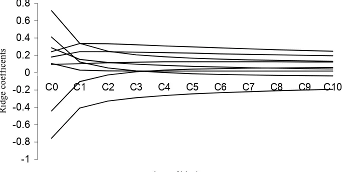
estimated ridge standardized regression coefficients for the different values of c, usually between 0 an 1. Extensive experience has indicated that the estimated regression coefficients bkR may fluctuate widely as c is changed slightly from 0,
and some may change signs. Gradually, however, these wide fluctuations cease and the magnitudes of the regression coefficients tend to move slowly towards zero as c is increased further. At the same time, the values of (VIF)k for k
regression coefficients on different biasing constants c tends to fall rapidly as c is changed from zero, and gradually the (VIF)k values also tend to change only
moderately as c increased further. Whereas (VIF)k is defined by Gruber (1998)
given in eq. (2.2) after correlation transformation (VIF)k =
1 1
) (
)
(rxx +cI − rxx rxx + cI − (2.2) Usually the plot of the estimated ridge standardized regression coefficients becomes stabilize and the (VIF)k value for each X variable becomes
approximately equal to one for the same value of biasing constant c. Hoeral et al. (1975) suggested another possible automatic way of choosing c. They argued that a reasonable choice might be given in eq. (2.3)
)} 0 ( { )}' 0 ( { ) 1 ( * * 2 b b S p
C = − (2.3)
Where (p-1) is the number of parameter in the model excluding intercept, S2 is the residual mean squares in the ANOVA table obtained from standard least square fit and {b* (0)}’ is given in eq. (2.4)
) 0 ( ),..., 0 ( ), 0 ( { } ),...., 0 ( ), 0 ( { )} 0 (
{b* ' = b1* b2* b(*p−1) = S11b1 S22b2 S(p−1)(p−1)b(p−1) (2.4)
After finalizing a forecasting model for wheat area significance of the explanatory factors is checked through modified t test explained by Gruber (1998) and given in eq. (2.5)
ii R
i
S b
t = ˆ (2.5)
Sii is the i’th diagonal element of the dispersion matrix of the ridge estimator given in eq. (2.6)
1 1 2 ) ( ) ( + − + −
= r cI r r cI
D σ xx xx xx (2.6)
Where σ2 is given in eq. (2.7)
) 1 ( ˆ ˆ 2 − − ′ = p n e e
σ (2.7)
Mallows Cp Statistic
examples of its use. Kennard (1971) showed that there is one-to-one correspondence between Cp and the adjusted R2.
The statistic is given by the formula:
Cp = (SSEp / MSEm) - (n-2p) (2.8)
Where SSEp is SSE for the best model with p parameters (including the intercept, if it is in the equation), and MSEm is the mean square error for the model with all m predictors. In general, we look for models where Cp is small and is also close to p. This is used in selection of best subset of predictors for forecasting model of Wheat production.
3. Results and Discussion
Assumptions of OLS estimation are checked. Ridge regression is used to correct multicollinearity problem in the data for wheat area models. The forecasting models are developed on the basis of 15 years data from 1984-85 to 1998-99 then wheat area and production for next five years from 1999-2000 to 2003-04 is forecasted through these models and compared with the actual figures. After evaluating the accuracy of models, final models are developed on the basis of 20 years for the period 1984-85 to 2003-04. These forecasting models can be used to forecast wheat area and production of next five years.
Tests for the assumptions of OLS estimation are performed and only the problem multicollinearity is found.
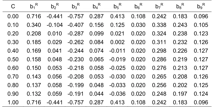
The ridge regression coefficients for biasing factor at 0 ≤ C ≤ 1 are given in Table No.1.
Table 1: Ridge Regression Coefficients
-1 -0.8 -0.6 -0.4 -0.2 0 0.2 0.4 0.6 0.8
C0 C1 C2 C3 C4 C5 C6 C7 C8 C9 C10
Values of biasing constat c
R
idge coef
fi
ce
nt
s
Ridge trace shows that the ridge standardized regression coefficients are stabilized between C1=0.10and C2=0.20.
VIF for all ridge standardized regression coefficients at different values of Ci
between 0.10 and 0.20 are given in table No. 2.
Table 2: VIF For C=0.10 to C=0.19
C VIF1 VIF2 VIF3 VIF4 VIF5 VIF6 VIF7 VIF8 VIF9 ∑VIFi 0.11 1.422 1.498 1.352 1.374 1.603 1.335 1.244 1.346 1.507 12.681 0.12 1.297 1.391 1.251 1.301 1.489 1.265 1.179 1.284 1.379 11.836 0.13 1.190 1.297 1.163 1.235 1.389 1.202 1.120 1.227 1.268 11.091 0.14 1.098 1.214 1.086 1.175 1.299 1.145 1.067 1.175 1.172 10.429 0.15 1.017 1.140 1.018 1.120 1.218 1.092 1.019 1.126 1.088 9.837 0.16 0.946 1.073 0.958 1.069 1.145 1.044 0.975 1.080 1.013 9.304 0.17 0.884 1.013 0.904 1.023 1.080 0.999 0.935 1.038 0.947 8.823 0.18 0.828 0.958 0.856 0.980 1.020 0.958 0.898 0.998 0.889 8.385 0.19 0.779 0.909 0.813 0.940 0.966 0.920 0.863 0.961 0.836 7.986
Above table shows that better value of C lies between 0.16 and 0.17.
Therefore again VIFi at different values of Ci between 0.16 and 0.17 are
calculated and achieved an improved value of C= 0166.
Other way to choose C given at equation No. 3 is use where {b*(0)}/ = {28.39493, -17.47910, -29.99067, 11.37353, 16.35693, 4.26636, 9.60239, 7.24485, 3.79672}, S2 = 51.8976 and p-1 = 9, therefore C= 0.181.
Following is the wheat area model based on agricultural and meteorological data for the period 1984-85 to 1998-99 after transforming back to the original variables at biasing factor C = 0.166.
Y = 199.4309 + 0.23803X1 – 0.00185X2 – 7.41126X3 – 0.71843X4 + 0.64493X5
+ 0.03488X6 + 0.22574X7 + 0.11487X8 + 0.08677X9
The table No. 3 shows the forecasting ability of above wheat area model.
Table 3: Forecasting Wheat area
S. No. Year
Area Percentage
Difference Forecasted Actual
1 1999-2000 319.000 320.099 0.34
2 2000-01 306.000 309.688 1.21
3 2001-02 267.000 277.547 3.95
4 2002-03 273.000 274.648 0.60
5 2003-04 300.000 295.281 -1.57
In the light of above research study, final ridge regression model based on agricultural and meteorological data for the period 1984-85 to 2003-04 after transforming back to the original variables at biasing factor C = 0.166 is given below.
Y = 206.230 + 0.215X1 – 0.001X2 – 6.626X3 +0.410X4 + 0.6475X5 + 0.054X6
+ 0.210X7+ 0.129X8 + 0.091X9
The values of R2 and adjusted R2 for above model are 92.83% and 87.62% respectively. Therefore above model can be used successively for the estimation of wheat area of district Chakwal for next five years with greater accuracy, that is, for the period 2004-05 to 2008-9.
Modified t test is performed and the calculated values of t-statistic for standardized ridge regression coefficients at C = 0.166 are {40.9144, -5.1946, -61.1618, 21.9034, 11.2136, 11.9742, 61.8093, 37.4008, 18.5363}.
All explanatory variables playing significant role to explain area under wheat crop for Chakwal district.
Wheat production model
Tests for assumptions of OLS estimation are conducted and violation of assumption under consideration is not found in the data.
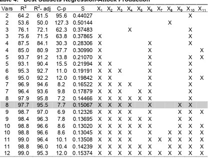
Best subsets regression
R2, Adj-R2, C-p and S are given table No. 4.
Table 4: Best Subsets Regression-Attock Production Vars R2 R2- adj C-p S X
1 X2 X3 X4 X5 X6 X7 X8 X9 X10 X11
2 64.2 61.5 95.6 0.44027 X
2 53.6 50.0 127.3 0.50144 X
3 76.1 72.1 62.3 0.37483 X X
3 75.6 71.5 63.8 0.37865 X X
4 87.5 84.1 30.3 0.28306 X X X
4 85.0 80.9 37.7 0.30990 X X X
5 93.7 91.2 13.8 0.21070 X X X X
5 93.1 90.4 15.5 0.21994 X X X X 6 95.3 92.7 11.0 0.19191 X X X X X 6 95.0 92.2 12.0 0.19842 X X X X X 7 96.9 94.6 8.2 0.16522 X X X X X X 7 96.4 93.6 9.8 0.17879 X X X X X X 8 97.9 95.8 7.2 0.14466 X X X X X X X
8 97.7 95.5 7.7 0.15067 X X X X X X X
9 98.7 97.0 6.9 0.12326 X X X X X X X X 9 98.4 96.3 7.8 0.13695 X X X X X X X X 10 98.8 96.6 8.6 0.13020 X X X X X X X X X 10 98.8 96.6 8.6 0.13045 X X X X X X X X X 11 99.0 96.4 10.1 0.13508 X X X X X X X X X X 11 98.8 96.0 10.4 0.14239 X X X X X X X X X X 12 99.0 95.3 12.0 0.15374 X X X X X X X X X X X
Keeping in view these results, the explanatory variables X1, X2, X3, X4, X6, X9 and
X10 are recommended to forecasting of wheat production. Analysis of regression
coefficients is given in table No. 5.
Table 5: Regression Analysis
Predictor Coef StDev T P
Constant 6.28700 1.51300 4.16 0.004 X1 0.09555 0.02898 3.30 0.013 X2 0.09038 0.02104 4.30 0.004 X3 2.80000 0.98410 2.85 0.025 X4 0.53360 0.19370 2.75 0.028 X6 0.01430 0.00256 5.58 0.000 X9 0.00895 0.00553 1.62 0.150 X10 -0.30702 0.04742 -6.47 0.000
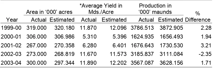
Forecasting of wheat production in thousand maunds for the period 1998-99 to 2002-2003 and percentage increase/decrease of forecasted production over actual production is calculated and given in table No. 6.
Table 6: Forecasting of Wheat Production
Year
Area in ‘000’ acres
*Average Yield in Mds./Acre
Production in
‘000’ maunds % Difference Actual Estimated Actual Estimated Actual Estimated
1999-00 319.000 320.180 11.870 12.096 3786.513 3872.905 2.28 2000-01 306.000 306.986 5.310 5.396 1624.935 1656.493 1.94 2001-02 267.000 270.358 6.280 6.401 1676.643 1730.530 3.21 2002-03 273.000 268.819 11.670 11.573 3185.837 3111.084 -2.35 2003-04 300.000 297.344 11.890 12.202 3567.087 3628.156 1.71
* Average yield in Mds./Acre = 3.89024 x Average yield per plot
Again the regression coefficients are calculated on the basis of agricultural and meteorological data for the period 1984-85 to 2003-04. The forecasting model with these regression coefficients is given below:
Y = 6.30000 + 0.09315X1 + 0.09201X2+ 2.88820X3 + 0.54664X4 + 0.01440X6
+ 0.00943X9 - 0.31118X10
This can be used successfully to forecast wheat production for the period 2004-05 to 2008-09.
3. Conclusion
The Urea fertilizer, DAP fertilizer and manures plays a significant role to enhance the production of wheat crop. Number of ploughs in the wheat fields is significant factor to increase the production of wheat crop. Good rains in the month of October and November significantly contributes to increase the production of wheat crop and mean maximum temperature in the month of March is a significant factor to reduce the production of wheat crop. All explanatory variables involved in the model playing their role to forecast the wheat production according to the prior expectations of agriculturists.
Recommendations
• Collection, tabulation and computerization of agricultural and agro-meteorological statistics. The Agriculture Statistics includes results of acreage, yield estimation surveys, support prices, harvest prices and market prices of agricultural commodities and off-take of fertilizers whereas Agro-metrological Statistics include temperature, humidity, rainfall, air pressure, winds and storms.
• Level of impact of these factors on different stages of crop development should be quantified. On the basis of these factors area and production forecasting models should be developed for all major as well as minor crops.
• Validity of these forecasting models should be evaluated on the basis of the results of objective surveys. Day by day improvement of these models should be a regular job of this section.
References
1. Gorman and Toman (1966), “Selection of variables for fitting equations to data”, Technometrics, 8(3), 27-51.
2. Gruber, M. H. J. (1998), “Improving Efficiency by Shrinkage”, Marcel Dekker, Inc. New York.
3. Hoerl, A. E. (1962), “Application of Ridge Analysis for Regression Problems”, Chemical Engineering Progress, 58(3), pp 54-59.
4. Hoerl, A. E. & Kennard, R. W. (1970a), “Ridge Regression: Biased Estimation for Non-orthogonal Problems”, Technometrics, 12(1), pp 55-67. 5. Hoerl, A. E. & Kennard, R. W. (1970b), “Ridge Regression: Biased
Estimation for Non-orthogonal Problems”, Technometrics, 12(1), pp 69-93. 6. Hoerl, A. E., Kennard, R. W. & Baldwin, K. F. (1975), “Ridge Regression:
Some Simulations”, Communication in Statistics: Theory and Methods, 4(2), pp105-123.