Efficient algorithms in analyzing genomic data

(1)

Eﬃcient Algorithms in Analyzing Genomic Data

Feng Pan

A dissertation submitted to the faculty of the University of North Carolina at Chapel Hill in partial fulﬁllment of the requirements for the degree of Doctor of Philosophy in the Department of Computer Science.

Chapel Hill 2009

Approved by:

Wei Wang, Advisor

Leonard McMillan, Co-principal Reader

Fernando Pardo-Manuel de Villena, Reader

David Threadgill, Reader

(2)

c 2009 Feng Pan

(3)

Abstract

Feng Pan: Eﬃcient Algorithms in Analyzing Genomic Data. (Under the direction of Wei Wang.)

With the development of high-throughput and low-cost genotyping technologies, immense data can be cheaply and eﬃciently produced for various genetic studies. A typical dataset may contain hundreds of samples with millions of genotypes/haplotypes. In order to prevent data analysis from becoming a bottleneck, there is an evident need for fast and eﬃcient analysis methods.

My thesis focuses on two interesting and important genetic analyzing problems.

• Genome-wide Association mapping. The goal of genome wide association mapping is to identify genes or narrow regions in the genome which have significant statistical correlations to the given phenotypes. The discovery of these genes offers the potential for increased understanding of biological processes affecting phenotypes such as body weight and blood pressure.

• Sample selection for maximal Genetic Diversity. Given a large set of samples, it is usually more eﬃcient to ﬁrst conduct experiments on a small subset. Then the following question arises: What subset to use? There are many experimental scenarios where the ultimate objective is to maintain, or at least maximize, the genetic diversity within relatively small breeding populations.

In my thesis, I developed the following eﬃcient and eﬀective algorithms to address these problems.

• Phylogeny-based Genom-wide association mapping:

(4)

– TreeQA+: TreeQA+ inherits all the advantages of TreeQA. Moreover, it improves TreeQA by incorporating sample correlations into the association study.

• Sample selection for maximal genetic diversity:

– Sample Selection in biallelic SNP Data: Samples are selected based on their genetic diversity among a set of SNPs. Given a set of samples, the algorithms search for the minimum subset that retains all diversity (or a high percentage of diversity).

(5)

List of Tables

2.1 Summary of Notations . . . 20

4.1 Notation Summary . . . 66

4.2 Correlation Clusters Embedded in Syndata1,2 and 3. . . 82

4.3 Correlated Gene Subsets . . . 90

5.1 A Sample-Marker Matrix . . . 98

5.2 Perlegen Data: Comparing the 8-strain subsets of the Collaborative Cross with the maximum diversity solution found byESE . . . 119

5.3 Voting Data: Subsets of 5 Samples found by ESE that have coverage = 1 119 5.4 Voting Data: Accuracy of Classiﬁers based on full set and subsets . . . . 120

5.5 Jester Data: Number of qualiﬁed sample subsets and their sizes for given ρ121 6.1 Notations . . . 128

6.2 Clustering Accuracy on Mushroom Dataset, Compared with SUMMARY, tmax=4 . . . 135

(10)

List of Figures

1.1 Examples of immense biological data . . . 2

1.2 An example SNP data and its corresponding binary matrix . . . 5

1.3 Example of maximal compatible regions and perfect phylogenetic trees . 7 2.1 Example: a SNP dataset and a perfect phylogeny tree . . . 18

2.2 The TreeQA Algorithm . . . 24

2.3 A fragment of theT reegrouping tree after enumerating the tree in Figure 2.1 27 2.4 Comparison of SMA, HAM, HapMiner and TreeQA on the simulated data 31 2.5 Comparison of TreeLD and TreeQA on the simulated data . . . 32

2.6 Compare SMA, HAM and TreeQA on the mouse genotype data . . . 33

2.7 The perfect phylogeny at the peak point found by TreeQA in Figure 2.6. 34 3.1 The sample correlations aﬀect the signiﬁcance of the association. . . 37

3.2 A SNP dataset and a perfect phylogeny tree. . . 40

3.3 An exmaple subtree with t branches. . . 41

3.4 General case groupings.. . . 45

3.5 Comparison of SMA, HAM, HapMiner, TreeLD, TreeQA and TreeQA+ on the simulated data. . . 54

3.6 Compare HAM, TreeQA and TreeQA+ on the mouse genotype data . . . 55

3.7 The two phylogenies at the peaks found by TreeQA and TreeQA+ respec-tively in Figure 3.6(b) . . . 56

4.1 Example Data . . . 59

(11)

4.3 Trees T{f1}_, _T{f2} _and _T{f4,f5} _{of the data matrix in Figure 4.2, with}

gmin = 1 . . . 64

4.4 Correlation: featuref₃ and groupings G₈{f1},P₁{f2} . . . 67

4.5 The TreeNL Algorithm . . . 73

4.6 RoutineTreeConstruct . . . 76

4.7 Re-designed RoutineEnumerateFeature+ . . . 77

4.8 Outputs of CURLER₄₀₀ and TreeNL on Syndata1 . . . 83

4.9 Outputs of CURLER₁₀₀ and TreeNL on Syndata2 . . . 84

4.10 Outputs of CURLER₁₀₀ and TreeNL on Syndata3 . . . 85

4.11 Clusters of objects found by TreeNL on Syndata3 . . . 86

4.12 Outputs of CURLER₂₀₀ and TreeNL on the NBA dataset . . . 87

4.13 Correlation clusters corresponding to correlated feature subsets 1 and 2 . 88 4.14 Outputs of CURLER₄₂ and TreeNL on the Mouse Gene Expression dataset 89 4.15 Correlation clusters of samples correspond to gene subsets in Table 4.3 . 90 4.16 Runtime comparison of CURLER₃₀₀, CARE, TreeNL and TreeNL+ on datasets of various sizes . . . 91

4.17 Runtimes of TreeNL and TreeNL+ when varying f setmax and gmin . . . . 92

5.1 The ESE Algorithm . . . 103

5.2 The P GDS Algorithm . . . 104

5.3 Enumeration Tree of the Matrix in Table 5.1 . . . 105

5.4 The KρDS Algorithm . . . 106

5.5 Scalability: Runtime on Synthetic Data . . . 115

5.6 Scalability: Runtime on Real Data . . . 115

5.7 Comparison of Subsets . . . 116

(12)

5.9 Perlegen Data: Distribution of Diversity Coverage of 8-sample Subsets. . 119

6.1 Example Data . . . 125

6.2 Mushroom dataset, tmax = 4, cmax = 4 . . . 134

6.3 Mushroom dataset, tmax = 3,cmax = 3 . . . 134

6.4 Runtime of diﬀerent tmin . . . 136

6.5 Number of candidates of diﬀerent tmin . . . 136

6.6 Diﬀerent tmin on Mushroom Dataset . . . 137

6.7 Mini 20 newsgroup,tmax <1, cmax = 1.1 . . . 138

6.8 Performance of 60 representatives . . . 138

(13)

Chapter 1 Introduction

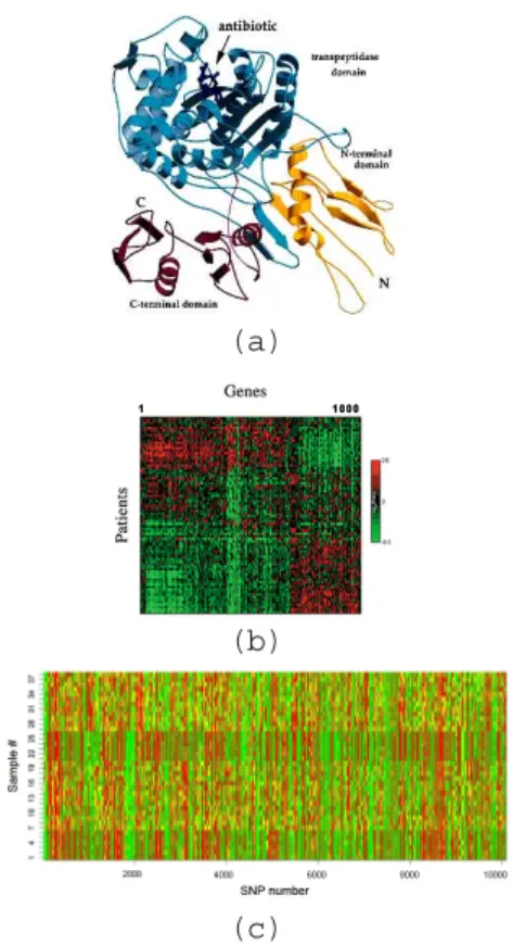
Genetics is the study of inheritance and variation in living organisms. A central dogma of modern genetics is that DNA is a template for making RNA which encodes the linear structure of proteins. Thus, biological data such as genomic data and proteomic data are frequently used in modern genetic analysis. In the early years of genetic study, getting sufficient data was the bottle neck of the analysis. Because of the high-cost and low-efficiency of sequencing technologies, scientists only have limited data, e.g. sparse genetic maps. Such data constrain the power of the various genomic analysis. Recently, with the development of high-throughput and low-cost sequencing technologies, immense biological data can now be cheaply and efficiently produced for various genetic studies. A few example datasets are shown in Figure1.1.

• In Figure 1.1 (a), a protein structural data contains the 3D information for

hun-dreds of amino acid.

• In Figure 1.1 (b), a microarray gene expression data contains thousands of gene

expression measurements from diﬀerent organisms or under diﬀerent environments.

• In Figure1.1 (c), a SNP (Single Nucleotide Polymorphism) data contains millions

(14)

(a)

(b)

(c)

Figure 1.1: Examples of immense biological data

These data are broadly used in biological analysis such as Quantitative Traits Loci Analysis (QTL), Gene Regulatory Network, and Protein Family Analysis.

While the immense genomic data are improving the power of various biological anal-ysis, they are also posing great computational challenges to the analysis studies. In QTL mapping, single marker analysis method (Pe’er et al. (2006); Akey et al. (2001)) is fast and frequently used. In a genomic dataset containing millions of markers, one scan of the single marker analysis method already takes hours to ﬁnish. Other com-plex methods such as haplotype-based mapping (McClurg et al. (2006); Onkamo et al.

(2002);Wang and Paigen (2005)) and phylogeny-based mapping (Zollner and Pritchard

(15)

the signiﬁcant threshold, the total number of tests can be further increased by a factor of 103 or even more.

Therefore, there is an urgent need to improve the eﬃciency and scalability of genetic study. The goal of my thesis is to develop eﬃcient analysis methods for various applica-tions in genetics. My thesis focuses on two interesting and important genetic analyzing problems as following:

1. Phylogeny-based Genome-Wide Association Mapping: The goal of genome wide association (GWA) mapping in modern genetics is to identify genes or nar-row regions in the genome that contribute to genetically complex traits such as morphology or diseases. Among the existing methods, phylogeny-based associa-tion mapping methods (Zollner and Pritchard(2005);Mailund et al.(2006);Sevon et al. (2006)) show obvious advantages over single marker-based methods (Pe’er et al. (2006); Akey et al. (2001)) and haplotype-based methods (McClurg et al.

(2006); Onkamo et al. (2002); Wang and Paigen (2005)) because they incorpo-rate information about the evolutionary history of the genome into the analysis. However, both the phylogeny inference and the more complex model indicted by the phylogeny cause the existing phylogeny-based methods to be far more time-consuming than single marker and haplotype-based methods. Methods such as TreeLD (Zollner and Pritchard(2005)) can take hours to analyze a small dataset containing tens of samples and markers. Thus, eﬃcient algorithms are in need for genome-wide scale analysis.

(16)

re-tention. A similar problem occurs when staging association studies across an RIL panel regarding how to order experiments in such a way that the most informa-tion is obtained. The problem of ﬁnding the sample subset having the greatest diversity is NP-complete. Given n samples, the problem has a searching space of size O(2n_{). A typical SNP dataset can contain hundreds of samples which makes}

it infeasible to perform a manual search. Eﬃcient algorithms which are optimized in runtime by heuristic searching are needed to handle the problem on real data.

In fact, the sample selection problem is closely related to the genome-wide association mapping problem. Genetic (allele) diversity is an important aspect to consider when designing association mapping studies. Sample selection could take place in the following two stages of GWA:

• Design of breeding program: In many cases, association mapping is conducted on

a population bred from a small set of samples. Usually, the number of available samples is larger than the number of samples needed to start a breeding program. A subset of samples which has the maximal genetic diversity is usually preferred over a random subset.

• Pre-processing of association mapping: A large set of samples cause computation

problems such as the huge number of permutation tests. By selecting a subset of the samples based on their genetic diversity, association mapping can be conducted more eﬃciently with no signiﬁcant loss in analysis capability. It also alleviates to some extent the bias caused by population distribution.

(17)

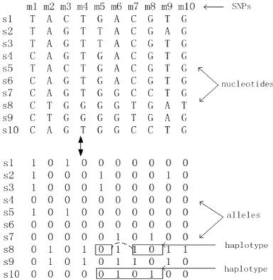
Figure 1.2: An example SNP data and its corresponding binary matrix

Nucleotide Polymorphisms (SNPs) are used as genetic markers. A SNP is a single nu-cleotide in the genome which diﬀers between individuals of a species (or between paired chromosomes in an individual). The variants of a SNP are called alleles. Previous work (Ideraabdullah et al.(2004)) has shown that over 99% of SNPs in mouse isogenic strains are biallelic (i.e., have two alleles), which allows us to represent allele diversity as a binary matrix. Figure 1.2 shows an example SNP data consisting of 10 sample chro-mosomes {s₁, s₂, ..., s₁₀} and 10 SNPs {m₁, m₂, ..., m₁₀}, and its corresponding binary matrix.

(18)

1.1 Eﬃcient Phylogeny-based Genome-wide

Associ-ation Mapping Algorithms

Previous studies (Zollner and Pritchard (2005); Mailund et al. (2006); Sevon et al.

(2006)) have shown that phylogeny-based association mapping methods outperform single-marker and haplotype-based methods. However, those phylogeny-based meth-ods (Zollner and Pritchard (2005); Mailund et al. (2006); Sevon et al. (2006)) are time-consuming and unable to handle real SNP data. In my thesis, I developed two eﬃcient phylogeny-based association mapping methods, TreeQA (Pan et al. (2009)) and TreeQA+. Instead of utilizing maximum-parsimony phylogeny or other types of phylogenies (which takes a long time to be inferred from genomic data), TreeQA and TreeQA+ examine the association between the inferred local perfect phylogenetic trees and the phenotype. A perfect phylogenetic tree (Fernandez-Baca (2001)) demonstrates the genetic relationship among a set of haplotypes. For any given set of haplotypes, a unique perfect phylogenetic tree exists if and only if the haplotypes are from a compat-ible region.

Given a SNP data and a phenotype, both TreeQA and TreeQA+ algorithms take three steps:

1. Identify maximum compatible regions in the SNP data: A compatible region con-sists of a set of consecutive SNP markers which are all pair-wise compatible by the 4-gamet rule (Hudson and Kaplan (1985)). All genetic variances in a compatible region are introduced by mutations, not from recombination or homoplasy. Each compatible region is maximized on both sides so that it contains as much genetic information as possible.

(19)

Figure 1.3: Example of maximal compatible regions and perfect phylogenetic trees

et al. (1995)). A piece of SNP data, the identiﬁed maximal compatible regions and their corresponding perfect phylogenetic trees are shown in Figure 1.3.

3. Examine the association between each tree and the phenotype: By removing com-binations of edges of the tree, both TreeQA and TreeQA+ enumerate all partitions indicated by each tree, but use diﬀerent statistical models and methods to examine the association between each partition and the phenotype.

In Step 3 of the above framework, genetic relationships among the samples are incor-porated into the association analysis by examining all the partitions of samples indicated by the perfect phylogenetic trees. TreeQA and TreeQA+ utilize diﬀerent models and tests to examine the partitions:

• TreeQA utilizes F-test and permutation test to calculate the signiﬁcance of the

(20)

• TreeQA+ improves TreeQA by utilizing the Brownian motion and maximum

like-lihood model to incorporate sample correlations induced by trees. The correlations violate the sample independence assumption and can bias the signiﬁcance of the association. Ignoring the correlations may cause spurious association to be de-tected.

Even though both TreeQA and TreeQA+ utilize a linear-time tree inference algo-rithm, they are still facing the computational challenges caused by test calculation and permutation test. Several eﬃciency optimizations are developed in the two algorithms.

In particular, for TreeQA:

1. Identical partitions indicated by diﬀerent trees are stored and retrieved in a preﬁx tree. The association score of a partition is only calculated once.

2. The intermediate computations in permutation tests are maximally reused by re-designing the calculation.

And for TreeQA+:

1. The number of permutations conducted in each permutation test is varied based on the current best association.

2. The calculation in the maximum likelihood model is optimized to avoid repeated calculations.

In my thesis, extensive experiments are conducted on both synthetic and real SNP data. The results show that TreeQA and TreeQA+ are more robust and eﬀective than single marker and haplotype-based methods, and are more eﬃcient than the previous phylogeny-based methods such as TreeLD (Zollner and Pritchard (2005)).

(21)

correlated with each other, e.g., a target feature has dependency on other features. This extended application diﬀers from TreeQA in the following three aspects.

1. Hierarchy clustering algorithms are used to generate the tree structures represent-ing sample relationships.

2. All feature subsets are considered in the association test, instead of only consid-ering consecutive features.

3. Every feature is considered as a potential target feature (which may have depen-dency on other features).

In my thesis, I applied TreeNL on real consensus data and found interesting corre-lated feature subsets.

1.2 Sample Selection based on Genetic Diversity

Sample selection is closely related to the genome-wide association mapping problem. In my thesis, the maximum-diversity sample selection is formalized as: select a minimum sample subset which can at least retainρ percent of the genetic diversity. In the studies, the genetic diversity is measured by the sample variation retained on the set of genetic markers. In a biallelic SNP dataset, the genetic diversity is measured as the percentage of SNP markers of which both alleles occur in the selected samples. In non-biallelic genomic data, the diversity is measured by information-theoretic measurements such as mutual information (Guiasu (1977)).

In my thesis, I ﬁrst developed algorithms to tackle the sample selection problem on biallelic SNP data. In this case, the problem of maximum-diversity sample selection is proved to be NP-complete via reduction from the Set Cover problem (Cormen et al.

(22)

Set Cover problem (Cormen et al. (2001)). It chooses the subset that maximizes the increase in coverage in each step until all the elements are covered. Therefore, I developed the PGDS (Pan et al.(2007)) algorithm which takes a similar greedy searching scheme.

PGDS chooses the sample that maximizes the increase in the diversity retained in each step. The PGDS algorithm is diﬀerent from the general Set Cover algorithm in two aspects:

1. PGDS is restarted with each sample and it picks the smallest subset from the n

subsets generated, wheren is the number of samples. Because a greedy algorithm cannot pick the best ﬁrst sample based on diversity since every single sample provides zero diversity.

2. The PGDS algorithm may stop once the genetic diversity retained in the selected sample subset exceeds the minimum threshold.

The PGDS algorithm is eﬃcient on real SNP data as demonstrated in my thesis. However, it does not guarantee the optimal solution. Therefore, I also developed an exhaustive-searching algorithm in my thesis, KρDS (Pan et al. (2007)), which is guar-anteed to get the optimal solution eﬃciently in biallelic SNP data. KρDS uses PGDS

as its pre-processing step. With the size of the possible minimum subset, K, reported by PGDS,KρDS searches all possible combinations of samples up to size K in an enu-meration tree. By imposing an order on the samples, the KρDS algorithm is able to perform a systematic search by enumerating all combinations, i.e., no combination is missed or revisited. Because of the exhaustive search scheme, KρDS guarantees to ﬁnd the optimal solution. In the worst case, the KρDS algorithm has a searching space of size O(2n_{) and takes exponential time. In order to accelerate the search, the} _KρDS

algorithm uses several pruning strategies to prune the searching space as follows:

• Dynamically Limit the Size of the Minimum Sample Subset: As mentioned above,

(23)

During the search, the value ofKis also updated to be the size of the smallest sub-set found so far (i.e.retains the minimum percentage of diversity). All remaining sample subsets of larger sizes can be pruned from the enumeration tree without further examination.

• Order Samples by Pair-wise Diversity: The runtime ofKρDS depends on how deep

it searches into the enumeration tree. KρDS can use less time to find the optimal solution if it can find a qualified subset in the earlier stages of the enumeration. Therefore, KρDS orders the samples at each level of the enumeration according to their pair-wise diversity so that it has a larger chance to find a qualified subset in the early stages.

• Estimate a Branch Upper Bound on Diversity: During the enumeration, KρDS

estimates the maximal diversity that can be found in the sample subsets in the current branch. An easy way to get a maximal diversity of a branch is to calculate the diversity of the sample subset consisting of all the samples which will be enumerated in that branch. Obviously, all the other sample subsets in the branch can only achieve lower diversities than this particular subset. Therefore, if the maximal diversity is less than the thresholdρ,KρDS can safely prune the branch.

• Reﬁne the Branch Upper Bound on Diversity: The maximal diversity of a branch

is overestimated when it is calculated using all the samples in the branch. With the knowledge of the size of the current minimum subset,K,KρDS can reﬁne the upper bound to be the maximal diversity of any K-sample subsets in the current branch.

(24)

BothKρDSandPGDS only work on biallelic SNP data. For non-biallelic data, I de-veloped an information-theoretic sample selection algorithm, REP (Pan et al.(2005a)), to search maximal diversity subsets. Mutual information (Guiasu (1977)) is used to measure the diversity retained in a sample subset. The REP algorithm takes a greedy scheme. In each step, it chooses the sample that can maximize the increase in mutual information until the percentage of mutual information retained exceeds a minimum threshold. Because of the monotonicity property of mutual information of a growing sample subset, the REP algorithm can always ﬁnd a sample that increases the mutual information in each step. Therefore, the algorithm is guaranteed to terminate in ﬁnite steps. Due to the greedy searching scheme, REP does not guarantee the optimal solu-tion. However, experiments in my thesis demonstrate that the sample subsets selected by REP are near optimal.

1.3 Thesis Statement

Eﬃcient and eﬀective algorithms can be developed for the following two analysis tasks on large genomic data.

• Phylogeny-based genome-wide association mapping: I developed the TreeQA and

TreeQA+ algorithms which are eﬃcient Phylogeny-based GWA methods. I also extended the idea to general data mining tasks and developed the TreeNL algo-rithm.

• Maximum-diversity sample selection: I developed eﬃcient algorithms for both

biallelic data (theKρDS and PGDS algorithms) and non-biallelic data (the REP

(25)

1.4 Thesis Outline

The thesis is organized as follows:

• The TreeQA algorithm is presented in Chapter 2.

• The TreeQA+ algorithm is presented in Chapter 3.

• The extended TreeQA algorithm, TreeNL, and its application in correlation

clus-tering are discussed in Chapter 4.

• The algorithms for maximum-diversity sample selection on biallelic SNP data are

presented in Chapter 5.

• The REP algorithm for maximum-diversity sample selection on non-biallelic data

is presented in Chapter 6.

(26)

Chapter 2 TreeQA: Phylogeny-based Genome-wide

Association Mapping

2.1 Introduction

Genome wide association (GWA) mapping locates genes or narrows regions in the genome that have signiﬁcant statistical connections to phenotypes of interest. The discovery of these genes and regions oﬀers the potential to increase understanding of biological processes controlling manifestation of phenotypes.

The most frequent genetic variants are single nucleotide polymorphisms (SNPs), in which a single nucleotide in the genome differs between individuals within a species. With the development of low-cost genotyping technologies, extensive SNP data can be cheaply and efficiently produced, which further increases the computational complexity of GWA mapping. Thus, there is an evident need for fast and effective GWA mapping methods.

Existing methods of association mapping look for similarities among samples (chro-mosomes, haplotypes, etc.) that are correlated with the phenotypes. If strong associ-ations are present, the variance of the phenotype within groups of similar samples is substantially smaller than the variance over all samples.

(27)

haplotype-based association mapping (Wang and Paigen (2005);Toivonen et al.(2000);

Waldron et al. (2005)), samples are grouped according to their genetic variation at a single marker or a set of markers. For case/control phenotypes, markers that can divide samples into (almost) pure classes are reported. Though these methods employ diﬀer-ent strategies for grouping samples, the derived groups are evaluated without further consideration of the intergroup similarities or alternate groupings.

In observation of this, tree-based association methods (Mailund et al. (2006);Sevon et al. (2006); Zollner and Pritchard (2005)) utilize phylogenies constructed over the samples. The phylogeny tree is a rich yet compact representation of genetic similarities of the samples. It provides sensible groupings of samples at multiple resolutions. However, the existing methods either handle only case/control phenotypes (Mailund et al.(2006);

Sevon et al. (2006)) or do not scale to GWA mapping (Zollner and Pritchard (2005)). In this chapter, we introduce TreeQA, a tree-based quantitative GWA mapping al-gorithm. TreeQA utilizes local perfect phylogeny trees constructed in genomic regions exhibiting no evidence of historical recombination by the 4-gamete test (Hudson and Kaplan(1985)). Given a perfect phylogeny, TreeQA evaluates all implied groupings and ﬁnds the strongest associations to the phenotype. Furthermore, TreeQA can identify and remove outliers during association analysis.

A brute-force implementation consists of a double loop: for every phylogeny tree, and for every grouping represented by the tree, we conduct a separate ANOVA test to measure its association to the phenotype, and keep track of the best groupings and trees. This approach is ineﬃcient and prone to multiple test errors (Miller(1981)). Both the number of trees and number of groupings per tree can be very large1. This large number of possible groupings requires many ANOVA tests, which is not only expensive computationally, but also gives rise to spurious associations2. Thus, permutation tests

1_{For example, the number of trees can exceed tens of thousands in a chromosome-wide association} study. And there are up to 22n−2groupings that can be generated from a tree of _nsamples.

(28)

are necessary to ensure the statistical signiﬁcance of the discovered associations, which will further increase the computational burden.

TreeQA exploits the following properties:

1. Groupings generated from the same tree obey a partial order, thus allowing reuse of intermediate computations.

2. A grouping may be derived from diﬀerent trees, but only need to be evaluated once.

3. Diﬀerent phenotype permutations may share a substantial number of common computations that need to be computed only once. Thus, TreeQA employs two preﬁx-tree structures (Cormen et al. (2001)) to organize all observed sample sub-sets and groupings to facilitate the caching and retrieval of reusable computations and guide the enumeration and evaluation of groupings.

As a result, TreeQA is able to handle quantitative GWA mapping very eﬃciently and is more eﬀective and robust in association mapping than previous methods.

2.2 Related Work

Single-marker association mapping (Pe’er et al.(2006);Akey et al.(2001)) considers the sample groupings induced independently by each single marker. Statistical tests such as χ2 and F-tests are used to measure the association between the phenotype and each grouping. These methods are computationally eﬃcient, however, they do not utilize the additional information content carried by haplotypes over single markers.

(29)

haplotype patterns in the data, upon which sample groupings are created and evalu-ated. HapMiner (Wang and Paigen (2005)) clusters samples using consecutive subsets of markers, and then assess the phenotype’s association strength.

The utility of local phylogenies in association mapping has been recently explored in TreeLD (Zollner and Pritchard (2005)), Blossoc (Mailund et al.(2006)), and TreeDT (Sevon et al. (2006)). These methods use trees to represent sample similarities. Their approach is to exhaustively examine all possible groupings implied by the given phy-logenies without explicitly excluding any outliers. Both Blossoc and TreeDT assume simple categorical (binary) phenotypes. TreeLD handles quantitative phenotypes but is not scalable to GWA analysis.

Some other work (Larribea et al.(2002);Morris et al.(2002);Minichiello and Durbin

(2006)) uses a global phylogeny structure, e.g., ancestral recombination graph, over all markers in association mapping. However, because of the high computational cost of global phylogeny construction, these methods are not scalable to genome-wide analysis.

2.3 Preliminaries

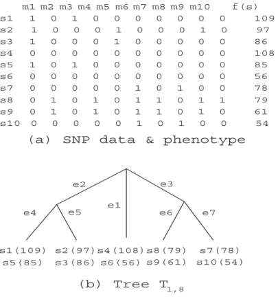
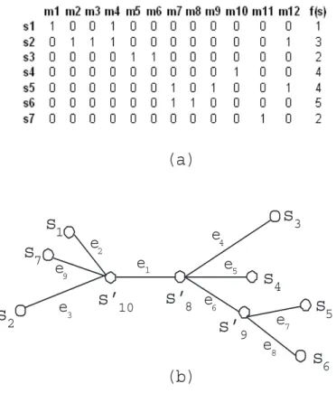
We use a binary matrixH =S×M to represent a SNP dataset, whereS ={s₁, s₂, ..., sn}

is the set of samples, and M = {m₁, m₂, ..., mz} is the SNP marker set. Each sample is represented by a binary vector, in which ’0’ represents the majority alleles and ’1’ represents the minority alleles. We usef(si) to denote the phenotype value of a sample si and F(S) to denote the phenotype values of samples in a subset S. An example

matrix H containing 10 samples and 10 SNP markers with phenotype is shown in Fig.

2.1(a).

(30)

m1 m2 m3 m4 m5 m6 m7 m8 m9 m10 f(s)

s1 1 0 1 0 0 0 0 0 0 0 109

s2 1 0 0 0 1 0 0 0 1 0 97

s3 1 0 0 0 1 0 0 0 0 0 86

s4 0 0 0 0 0 0 0 0 0 0 108

s5 1 0 1 0 0 0 0 0 0 0 85

s6 0 0 0 0 0 0 0 0 0 0 56

s7 0 0 0 0 0 1 0 1 0 0 78

s8 0 1 0 1 0 1 1 0 1 1 79

s9 0 1 0 1 0 1 1 0 1 0 61

s10 0 0 0 0 0 1 0 1 0 0 54

(a) SNP data & phenotype

(b) Tree T 1,8 s4(108) s6(56) s1(109) s5(85) s2(97) s3(86) s7(78) s10(54) s8(79) s9(61) e1 e2 e3

e4 e5 e6 e7

Figure 2.1: Example: a SNP dataset and a perfect phylogeny tree

the two markers, at most three of them occur.

A compatible region is a genomic region exhibiting no evidence of historical recom-bination. In Fig. 2.1(a), the region from markers m₁ tom₈ is a compatible region. We use Cu,v to denote a compatible region from markers mu to mv.

Deﬁnition 2.3.2. Maximal Compatible region: A compatible region is a maximal compatible region iﬀ it can not be extended on either side to include more SNPs and remains compatible.

Deﬁnition 2.3.3. Perfect Phylogeny Tree: A phylogeny tree for a set of samples is perfect if the phylogeny avoids homoplasy. Every SNP is introduced by a mutation and is represented by an edge of the tree. Given a genomic region, a perfect phylogeny exists iﬀ the region is a compatible region.

(31)

C₁,8 in Fig. 2.1(a), its tree T1,8 is shown in Fig. 2.1(b). All samples are at the leaf

nodes. Samples having identical haplotypes in the region share the same leaf node in the tree, e.g.,s₁ and s₅. Each internal node represents a hypothetical common ancestor of a subset of samples. Each edge uniquely corresponds to a SNP (or a historical mutation). Interested readers may refer to paper (Agarwala et al.(1995)) for inferring perfect phylogenies from a set of SNPs.

LetE(Tu,v) ={e1, e2, ..., ep}denote the set of edges inTu,v. The removal of each edge

partitions the samples into two subsets denoted byS(0)(ei) andS(1)(ei). Given a treeTu,v, we can generate 2|E(Tu,v)|sample subsets by removing each edge separately. We denote

this set of sample subsets byS(E)₍_T

u,v), S(E)(Tu,v) ={S(j)(ei)|j ={0,1}, ei∈E(Tu,v)}.

Deﬁnition 2.3.4. A grouping of a sample subsetS,G(S), is formed by a set of disjoint subsets of S, G(S) = {S₁, S₂, ..., S_k}, S_i ⊂S, S_i ∩S_j = ∅,k_i₌₁S_i =S. Given a tree

Tu,v, we say a groupingG(S) follows Tu,v iﬀ ∀S_i ∈G(S), S_i ∈S(E)(Tu,v).

For example, grouping G(S) = {{s₁, s₅, s₂, s₃},{s₈, s₉, s₇, s₁₀}} follows the tree in Fig. 2.1(b), while grouping G(S) ={{s₁, s₂},{s₈, s₄}}does not.

Deﬁnition 2.3.5. Given a sample subsetS,G₁(S) is called aparent-groupingofG₂(S) (G₂(S) called a child-groupingof G₁(S))iﬀ ∀S_i ∈G₁(S)

∃S_j ∈G₂(S), s.t.S_i =S_j. OR∃{S_j_q|S_j_q ∈G₂(S), q = 1, ..., u}, s.t.S_i =

u

q=1 S_j_q

A child-grouping represents a ﬁner partition of its parent-grouping on the same set of samples. For example, grouping {{s₁, s₅, s₂, s₃},{s₄, s₆}} is the parent-grouping of {{s₁, s₅},{s₂, s₃},{s₄, s₆}}. We summarize the notations in Table 4.1.

Association between a Compatible Region and a Phenotype

(32)

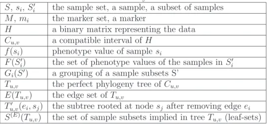
Table 2.1: Summary of Notations

S,si,S_i the sample set, a sample, a subset of samples

M, mi the marker set, a marker

H a binary matrix representing the data

Cu,v a compatible interval of H f(si) phenotype value of sample si

F(S_i) the set of phenotype values of the samples in S_i Gi(S) a grouping of a sample subsets S’

Tu,v the perfect phylogeny tree of Cu,v E(Tu,v) the edge set of Tu,v

T_u,v (ei, sj) the subtree rooted at node sj after removing edgeei S(E)₍_T

u,v) the set of sample subsets implied in tree Tu,v (leaf-sets)

re-derive the formula of the ANOVA test.

Given a grouping G(S) ={S₁, ..., S_k}, for every S_i ∈G(S), we calculate

SQ(S_i) =

s_j∈S_i

f(sj)2, SM(Si) =

s_j∈S_i

f(sj) (2.1)

SSEi =SQ(S_i)−SM(S_i)2/|S_i|, SSBi =SM(S_i)2/|S_i| (2.2)

Combining all subsets together, we have M M = _|_S1_|

k

i=1SM(Si) and

M SE= 1

|S| −k k

i=1

SSEi, M SB= 1

k−1(

k

i=1

SSBi− |S| ·M M2) (2.3)

We obtain a base score for grouping G(S)

0(G(S)) = M SB_{M SE} (2.4)

A higher score indicates a stronger association between the grouping and the pheno-type. Given the tree and the data in Fig. 2.1and the following two groupings: G(S₁) = {{s₂, s₃},{s₄, s₆},{s₈, s₉}}, G(S₂) = {{s₂, s₃},{s₈, s₉}}, the scores are ₀(G(S₁)) =

(33)

phenotype than groupingG(S₁).

To correct the multiple test errors, we apply a permutation test onG(S) to calculate a signiﬁcance score. To permute the phenotype, the phenotype values in F(S) are randomly re-assigned to samples inS. Then we calculate an-score using the permuted phenotype following Eqs. 5.1 to3.13.

Assume that we conductnPerm random permutations in total, for each permutation, we get score j(j = 1...nP erm). Among the nP erm -scores, let p be the number of

scores which are greater than or equal to the base score ₀(G(S)), i.e., p=|{j|j ≥

0(G(S)), j ∈1...nP erm}|. Then the signiﬁcant score (P score) ofG(S) is

P(G(S)) = log₁₀

nP erm p

(2.5)

A higher P score indicates that the association between grouping G(S) and the phenotype is more signiﬁcant.

Deﬁnition 2.3.6. The association between a compatible region and a phe-notype: For a compatible region Cu,v, the highest P score achieved by any grouping

following Tu,v is regarded as theP score ofCu,v. The P score represents the association

between the compatible region and the phenotype,

P(Cu,v) =max{P(Gj(S))|∀Gj(S)f ollows Tu,v, S ⊆S}. (2.6)

Problem Deﬁnition: Given a SNP data and a quantitative phenotype, calculate the

P-score of every maximal compatible region and report the most signiﬁcant ones.

2.4 TreeQA Algorithm

TreeQA takes two major steps:

(34)

phy-logenies of the regions.

2. Compute the association between each compatible region and the phenotype.

2.4.1 Maximal Compatible Region and Phylogeny

Construc-tion

TreeQA scans the SNP markers in a left to right order. In order to ﬁnd the maximal compatible regions, it continuously extends the current region by adding the next marker until the new marker is incompatible with some markers in the region. And it maximizes the overlap between two consecutive regions. Assume that the current compatible region isCu,v, and markermv+1 is incompatible with markersmi1, ..., mi_k,u≤i1 < ... < ik≤v,

then TreeQA starts the next compatible region at marker mi_k₊₁. For each maximal compatible region, TreeQA utilizes the inferring algorithm Agarwala et al. (1995) to construct a local perfect phylogeny tree. Both procedures have linear time complexity with respect to the number of markers and the number of samples.

2.4.2 Association Computing

In the second step, TreeQA takes as input a quantitative phenotype and a set of local perfect phylogenies. It considers all possible groupings following the phylogenies and systematically explores the search space of these groupings in a carefully designed order such that intermediate computations can be maximally reused.

According to Deﬁnition 2.3.4, any grouping of a sample subset3 that follows a tree

Tu,v can be created from non-overlapping subsets in S(E)(Tu,v). By utilizing the

lex-icographical order4 of subsets in S(E)₍_T

u,v), TreeQA can enumerate and evaluate all

combinations of non-overlapping subsets systematically.

3_{Considering groupings of a sample subset allows TreeQA to exclude potential outliers from the} ANOVA test.

(35)

TreeQA enumerates all groupings via a depth-ﬁrst recursive procedure. TreeQA ex-tends the current grouping by including a new sample subset which does not overlap with any subsets in the current grouping. The association of each new grouping to the phenotype via a permutation test is computed. The P score of the corresponding max-imal compatible region is updated accordingly. The enumeration continues recursively for each newly extended grouping.

Consider the tree in Figure 2.1. There are 14 sample subsets in S(E)(T₁,8). Assume

that the subsets have the following order,

se1 ={s1, s5}, se2=S−se1,se3 ={s2, s3}, se4 =S−se3, se5 ={s4, s6}

se6 =S−se5, se7 ={s8, s9}, se8 =S−se7, se9 ={s7, s10}, se10=S−se9

se11={s1, s5, s2, s3}, se12=S−se11, se13={s8, s9, s7, s10}, se14=S−se13

TreeQA ﬁrst generates a grouping containingse₁ only. Among the remaining sample subsets, {se₂, se₃, se₅, se₇, se₉, se₁₂, se₁₃} do not overlap with se₁. In the next step, a grouping {se₁, se₂} is formed by adding se₂ into the current grouping and its P score is calculated. P(C₁,8) is updated accordingly. Since all other sample subsets overlap

withse₁ orse₂. Thus, no new grouping can be extended from{se₁, se₂}. Then, TreeQA examines the next grouping extended from{se₁},{se₁, se₃}, and all groupings extended from it. After examining all groupings containing se₁, TreeQA will start from the grouping {se₂} and extend it recursively to generate all groupings containing se₂ but not se₁. This process continues until all distinct groupings are enumerated.

The pseudocode code of TreeQA is in Fig. 2.2.

2.4.3 Eﬀective Permutation

(36)

(37)

domly re-assigning the phenotype values in F(S) to samples in S; 2) calculating the corresponding score by Eq. 3.13.

Given a subsetS, both steps takeO(|S|) time. TreeQA exploits maximal reusability of intermediate computation shared by permutation through the following two optimiza-tions:

1)inTree: Common computation units shared by permutation tests of parent/child-groupings in a tree.

2)amgTree: Common computation units shared by permutation tests on groupings following multiple trees.

We use two global preﬁx-tree structures (Cormen et al. (2001)), T reegrouping and T reesubset to organize groupings and sample subsets examined thus far respectively to

enable eﬀective permutation tests.

inTree: Eﬀective permutation tests within a tree

A pair of parent/child-groupings always involve the same set of samples. Let S denote a set of samples. For the permutation tests of the parent/child groupings of S, instead of re-assigning the phenotype values in F(S) independently for each grouping, they can share the same set of random permutations ofF(S).

For example, given the example in Fig. 2.1 and a pair of parent/child-groupings,

G₁(S) ={{s₁, s₅, s₂, s₃},{s₈, s₉, s₇, s₁₀}}andG₂(S) = {{s₁, s₅},{s₂, s₃},{s₈, s₉, s₇, s₁₀}}, their₀ scores are: ₀(G₁(S)) = 9.79 and₀(G₂(S)) = 4.32. Assume that after a ran-dom permutation, the new phenotype values for the samples are: f(s₁) = 85,f(s₂) = 79,

f(s₃) = 109,f(s₅) = 61,f(s₇) = 86,f(s₈) = 97,f(s₉) = 78,f(s₁₀) = 54. Using this new assignment, we can calculate the newscores for both groupings: (G₁(S)) = 0.12 and (G₂(S)) = 0.7. By reusing the phenotype permutation between G₁(S) and G₂(S),

we save O(|S|) runtime in each permutation.

(38)

We say a grouping is at the ﬁnest level if it does not have any child-groupings. For example, given the tree in Fig. 2.1(b) and the two groupings G₁(S) and G₂(S) used above, grouping

G₃(S) ={{s₁, s₅},{s₂, s₃},{s₈, s₉},{s₇, s₁₀}}

is the child-grouping of both G₁(S) and G₂(S) and is at the ﬁnest level while G₂(S) is a ﬁner partition ofG₁(S).

We use a global preﬁx-tree T reegrouping to index all groupings and maintain the

parent/child relationship through auxiliary links (from a child-grouping to its parent-groupings). For each permutation of the phenotype, the scores of a finest grouping and all of its parent-groupings are calculated together. We examine the finest grouping immediately followed by the examination of its parent groupings for maximum compu-tation reuse. If a finest child-grouping has nparent-groupings, we save O(n|S|) time in each permutation.

Given a tree Ti, each grouping Gj(S) is inserted into or retrieved from T reegrouping

after Step 2 inEnumerate(). IfGj(S) exists in T reegrouping and theP score is already calculated which means Gj(S) has been examined, amgTree is used and the subroutine

jumps to Step 9 (discussion about amgTree is in Section 2.4.3). If grouping Gj(S) is

new, we insert Gj(S) into T reegrouping and generate its child-groupings recursively till

the ﬁnest level, say Gl(S).

If Gl(S) exists in T reegrouping (that is, it was examined before), we insert the new

leaf node of Gj(S) to the linked list headed by the leaf node of Gl(S). If Gl(S) is

not in T reegrouping (that is, this is the ﬁrst time it is examined), we insert Gl(S) into

the tree ﬁrst, create a linked list headed by the new leaf node ofGl(S), and insert the leaf node ofGj(S) in the linked list. Since a parent-grouping may be inserted into tree T reegrouping before its child-groupings and a child-grouping could have multiple

(39)

Figure 2.3: A fragment of the T reegrouping tree after enumerating the tree in Figure 2.1

For example, given the tree in Figure 2.1, after enumerating all groupings, a frag-ment of T reegrouping is shown in Figure 2.3. Parent/child-groupings are in linked lists

represented by dotted arrows, of which the ﬁnest groupings (such as {se₁, se₃, se₇}) are at the head.

amgTree: Eﬀective permutation among trees

The same grouping occurs repeatedly in diﬀerent trees. We only need to compute itsP

score at its ﬁrst occurrence. We use T reegrouping to store and retrieve theP score of all

examined groupings. If the grouping formed by TreeQA can be found inT reegrouping, its P score is directly used. Otherwise, its P score is calculated and stored in T reegrouping.

Based on our experiments on real data, usingamgTreealone can reduce 40%−50% of the execution time. When usinginTree andamgTreetogether, we can reduce 70%−80% of the execution time.

2.4.4 Reuse of Intermediate Computation of Statistical Tests

(40)

discussion.

We employ a global preﬁx-tree T reesubset to keep track of all sample subsets in any

groupings examined thus far. Three values are stored at the leaf node corresponding to the subset S: (subset ID, SQ₀(S),SM₀(S)).

For example, given the 10 samples and their phenotype values in Fig. 2.1(a), we calculate the base score₀ of grouping G₁(S) = {{s₁, s₅},{s₂, s₃},{s₇, s₁₀}}.

SQ₀(S₁₁) = 19106, SQ₀(S₁₂) = 16805, SQ₀(S₁₃) = 9000.

SM₀(S₁₁) = 194, SM₀(S₁₂) = 183, SM₀(S₁₃) = 132.

0(G1(S)) = 547.17/212.17 = 2.58.

The SQ₀ and SM₀ values of the three subsets are then stored in T reesubset. Given

a parent-grouping of G₁(S), G₂(S) = {{s₁, s₅, s₂, s₃},{s₇, s₁₀}}, we can retrieve the values of SQ₀ and SM₀ and use them to calculate ₀(G₂(S)),

SQ₀(S₂₁) = SQ₀(S₁₁) +SQ₀(S₁₂) = 35911, SQ₀(S₂₂) =SQ₀(S₁₃).

SM₀(S₂₁) = SM₀(S₁₁) +SM₀(S₁₂) = 377, SM₀(S₂₂) =SM₀(S₁₃).

0(G2(S)) = 1064.08/166.69 = 6.38.

(41)

2.5 Experimental Results

We compare TreeQA with the following algorithms:

1. SMA, our implementation of the Single Marker Association algorithm (Pe’er et al.

(2006);Akey et al. (2001)).

2. HAM, our implementation of the Haplotype Association Mapping algorithm ( Mc-Clurg et al. (2006)) that slides a 3-SNP window through the genome

3. HapMiner (Wang and Paigen (2005)), downloaded from the website5.

4. TreeLD(Zollner and Pritchard (2005)), downloaded from the website6.

Both SMA and HAMuse the one-way ANOVA test for fair comparison.

QHPM (Onkamo et al.(2002)) is not used for comparison because it is not scalable to large data sets. Blossoc (Mailund et al. (2006)) and TreeDT (Sevon et al.(2006)) are not used because they require categorical phenotypes.

2.5.1 Experiments on Simulated Data

We use Coasim (Mailund et al.(2005)) to simulate 1000 sequences with scaled recombi-nation rateρ= 400 that corresponds roughly to 10 cM. 10,000 SNP markers are placed uniformly at random over the sequences.

SNP markers on the sequences are randomly selected as causative loci with one, two and three causative mutations. The ﬁrst SNP is always selected randomly from all SNPs. In the cases of two and three mutations, the second and third causative SNPs are selected from compatible SNPs that are located less than 10 SNPs away from the ﬁrst SNP. Phenotype values are sampled from four Gaussian distributions: N₁(140,35),

(42)

N₂(90,35), N₃(50,40), and N₄(10,35). The one-mutation case uses N₁ and N₃. The two-mutation case usesN₁,N₂ and N₃. The three-mutation case uses all four Gaussian distributions. After assigning the phenotype values, all causative SNPs are removed from the data and we randomly select 100 sequences for our experiments.

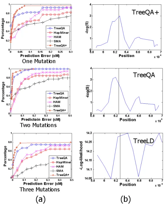
SMA, HAM and HapMiner output the top one scoring locus as a point estimation of the causative locus, while TreeQA outputs the top one compatible region. We compare the eﬀectiveness of the algorithms by measuring the distance (in cM) from the top one scoring locus or the center of the top one region to the causative SNP (or the average distance to every causative SNP). We call the distance the Prediction error.

Since HapMiner can not ﬁnish processing 10,000 SNP markers in a reasonable time, we only use the ﬁrst 1,000 markers of each sequence when applying HapMiner on the simulated data.

The comparison of SMA, HAM, HapMiner and TreeQA is shown in Figure 3.5. The x-axis represents the prediction error (distance) to the causative locus and the y-axis represents the percentage of causative loci which are found in distance less than x. In all three cases, the estimated loci by TreeQA are closer to the causative loci than those by SMA, HAM and HapMiner.

(43)

(44)

Figure 2.5: Comparison of TreeLD and TreeQA on the simulated data

locus while TreeLD identiﬁes one spurious peak.

2.5.2 Experiments on Mouse Genotype Data

We used a set of mouse genotypes that combines experimental and imputed data7 ( Sza-tkiewicz et al. (2008)) from the Jackson Laboratory, consisting of 74 samples. The dataset contains over 7 million SNP markers distributed over all 20 chromosomes. We removed wild derived mouse inbred strains since they are quantitatively and qualitatively diﬀerent than other laboratory inbred strains and we only used in our experiments the remaining 55 samples that have a share set of common ancestral relationships (Yang et al. (2007)).

We used high density lipoprotein cholesterol (HDL-C) levels in blood as the test phenotype, downloaded from the Mouse Phenome Database8. Several HDL-C datasets are available, each of which was collected under diﬀerent conditions, and are thus treated as separate phenotypes. Some candidate genes that may play a role in regulating HDL-C levels are reported in (Wang and Paigen (2002)).

7_{http://cgd.jax.org/ImputedSNPData/imputedSNPs.htm}

(45)

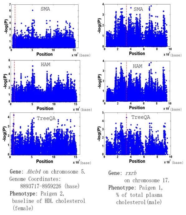
We apply SMA, HAM and TreeQA on the data and examine how close they can identify the top peak near the locus of those candidate genes.

SMA

(base)

TreeQA

(base)

HAM

(base)

SMA

(base)

HAM

(base)

TreeQA

(base)

Figure 2.6: Compare SMA, HAM and TreeQA on the mouse genotype data

(46)

129S1/SvImJ(63.8)

BTBRT<+>tf/J(72.9)

C58/J(65.4)

LP/J(50.2)

MA/MyJ(75.8)

NZB/BlNJ(100)

NZW/LacJ(90.9)

RF/J(77.6)

KK/HLJ(89.3)

A/J(45.3), AKR/J(44.9), BALB/cByJ(56.8), C3H/HeJ(75.8), C57BL/10J(44.6),

C57BL/6J(49.7), C57BLKS/J(36.7), C57BR/cdJ(67.8), CL/J(39.5), CBA/J(49.4),

DBA/1J(39.6), DBA/2J(43.3), I/LnJ(42.4), NON/LtJ(72.2), PL/J(51.7), RIIIS/

J(40.2), SEA/GnJ(52), SJL/J(40.6), SWR/J(46.8)

FVB/NJ(94.7)

NOD/LtJ(54.6)

BUB/BnJ(63.4)

SM/J(48)

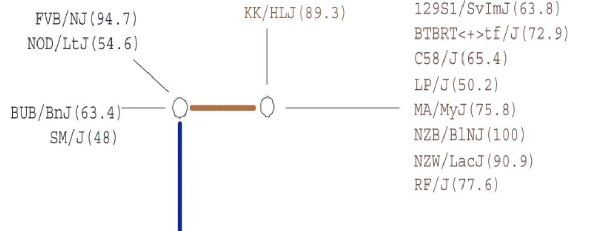
Figure 2.7: The perfect phylogeny at the peak point found by TreeQA in Figure 2.6

The perfect phylogeny corresponding to the peak point (compatible region from 8799298 to 8801558 (base)) found by TreeQA around Abcb4 in Figure 2.6 is plotted in Fig. 2.7. The phenotype values of the samples are in parentheses. Samples with unknown phenotype values are omitted from the tree. The subtree on the right contains samples having high phenotype values while the subtree at the bottom contains samples having low values. Other subtrees are considered as outliers and are excluded from the grouping. SMA and HAM fail to identify the locus because they only examine sample groupings that can be generated from single SNPs or 3-SNP windows, which are a small subset of the groupings examined by TreeQA.

(47)

2.6 Conclusion

(48)

Chapter 3 TreeQA+: Improving the Power of

Phylogeny-based Genome-wide Association

Mapping

3.1 Introduction

In Chapter 2, I discussed the TreeQA algorithm which is a phylogeny-based genome-wide association mapping method. The experimental results on both synthetic and real data demonstrates that TreeQA outperforms single marker-based and haplotype-based methods. TreeQA also outperforms the previous phylogeny-haplotype-based methods such as TreeLD, Blossoc and TreeDT (Zollner and Pritchard (2005); Mailund et al. (2006);

Sevon et al.(2006);Larribea et al.(2002); Morris et al. (2002);Minichiello and Durbin

(2006)) in terms of runtime and the ability to handle quantitative traits.

However, both TreeQA and other phylogeny-based methods do not consider the sample correlations implied by the tree topologies in the analysis. Ignoring sample correlations can bias the signiﬁcance of the associations and lead to spurious signals.

(49)

s1(20) s2(50) s3(10) s4(10) s5(10) s6(50)

(a)

s1(20) s2(50) s3(10) s6(50)

(b)

s1(20) s2(50) s3(10) s4(10) s5(10) s6(50)

(c)

20 20 20 20 20 20 20 20 20 20 20 20 20 20 20 20 19 1 1 1

Figure 3.1: The sample correlations aﬀect the signiﬁcance of the association.

get partitions,{{s₁, s₂},{s₃, s₆}},{{s₁, s₂},{s₃, s₄, s₅, s₆}}and{{s₁, s₂},{s₃, s₄, s₅, s₆}}

from the three trees. The mean phenotype values of the left group and right group in these partitions are, {35,30}, {35,20} and {35,20}. If all samples are assumed to be independent as in the previous methods, the associations between the partitions and the phenotype would be equally strong in trees (b) and (c), and weak in tree (a). However, since s₃, s₄ and s₅ are far more closely related to each other than to the remaining samples (indicated by the short branches between them) in tree (b), it is erroneous to treat them as independent samples in tree (b). In fact, the associations between the partitions and the phenotype should be similarly weak in trees (a) and (b), and relatively strong in tree (c).

Therefore, it is critical to take into account the sample correlations implied by the topology properly in association study. However, this is not a trivial task, especially when we assess the association of the partitions such as{{s₁, s₂},{s₃, s₄, s₅},{s₆}} (cre-ated by removing multiple edges).

(50)

which incorporates the sample correlations modelled by local perfect phylogeny trees. As a phylogeny-based method, TreeQA+inherits all advantages of TreeQA by examining all groupings induced by a perfect phylogeny (constructed in genomic regions exhibiting no evidence of historical recombination by the 4-gamete test(Hudson and Kaplan(1985))). In addition, TreeQA+ is more eﬀective and robust than TreeQA by incorporating sample correlations. TreeQA+ adopts the model of Brownian motion (Nelson (1967)) which was previously used to study phylogeny (Edwards and Cavalli-Sforza (1964);

Felsenstein (1981)): for any two nodes (samples or hypothetical ancestors) in the phy-logeny, if there is no causative mutation happened during the evolution from one node to the other, the diﬀerence between the phenotype values of the two nodes should fol-low a normal distribution with mean 0 and variance proportional to the sum of edge lengthes between them. Thus, any signiﬁcant deviation from this estimation suggests the existence of some causative mutations during the evolution.

In TreeQA+, a grouping also consists of several non-overlapping subtrees created by removing edges from a perfect phylogeny tree. TreeQA+ utilizes Felsenstein’s tree pruning method (Felsenstein (1981)) to estimate the phenotype values of hypothetical ancestors (intermediate nodes) in each subtree. Then the estimated phenotype values at the two adjacent nodes of each removed edge are examined under the assumption of Brownian motion. A signiﬁcant deviation between the two nodes implies a strong association between the grouping and the phenotype. For each phylogeny, TreeQA+ ﬁnds the strongest association between its induced groupings and the phenotype.

A brute-force implementation of TreeQA+ is computationally expensive. TreeQA+ faces the same computational challenge as TreeQA.

• Both the number of trees and number of groupings per tree can be very large1 in

a GWA mapping.

(51)

• Permutation tests are necessary to ensure the statistical signiﬁcance of the

discov-ered associations, which further increase the computational burden.

Since different statistical methods are used, the optimizations developed in TreeQA can not be used in TreeQA+. However, the same strategy applies, i.e., maximize the reuse of intermediate computations. A few new optimizations are developed and make TreeQA+ very efficient and effective in GWA mapping, as demonstrated by extensive experiments on both simulated datasets and inbred mouse strains.

3.2 TreeQA

+

Method

3.2.1 Preliminaries

In this chapter, we use the same set of designations and deﬁnitions (e.g., maximum compatible interval and grouping induced by a tree) as in Chapter 2. Fig. 4.2 shows an example matrix H containing 12 SNP markers, one phenotype for 7 samples and a perfect phylogenetic tree. We use this example matrix and tree as the running example in this section.

(b)

s

₇

e

9

Figure 3.2: A SNP dataset and a perfect phylogeny tree.

association between the partition and the phenotype values by comparing the means and variances of the partitions using a t-test or f-test. However, as discussed in Section

3.1, this approach ignores the sample correlations in each subset.

In contrast, TreeQA+ incorporates sample correlations into the association test. Given a grouping, TreeQA+ estimates the expected phenotype value of the root node of each subtree from the phenotype values of the leaf nodes and the topology of the subtree by utilizing Felsenstein’s tree pruning algorithm (Felsenstein (1981)). Then the association between the grouping and the phenotype is measured by examining the dif-ferences between these estimated phenotype values separated by the removed edges in a Brownian motion (Nelson (1967) model).

Efficient algorithms in analyzing genomic data

Eﬃcient Algorithms in Analyzing Genomic Data

Abstract

Table of Contents

List of Tables

List of Figures

Chapter 1

Introduction

1.1

Eﬃcient Phylogeny-based Genome-wide

Associ-ation Mapping Algorithms

1.2

Sample Selection based on Genetic Diversity

1.3

Thesis Statement

1.4

Thesis Outline

Chapter 2

TreeQA: Phylogeny-based Genome-wide

Association Mapping

2.1

Introduction

2.2

Related Work

2.3

Preliminaries

Association between a Compatible Region and a Phenotype

2.4

TreeQA Algorithm

2.4.1

Maximal Compatible Region and Phylogeny

Construc-tion

2.4.2

Association Computing

2.4.3

Eﬀective Permutation

2.4.4

Reuse of Intermediate Computation of Statistical Tests

2.5

Experimental Results

2.5.1

Experiments on Simulated Data

2.5.2

Experiments on Mouse Genotype Data

129S1/SvImJ(63.8)

BTBRT<+>tf/J(72.9)

C58/J(65.4)

LP/J(50.2)

MA/MyJ(75.8)

NZB/BlNJ(100)

NZW/LacJ(90.9)

RF/J(77.6)

KK/HLJ(89.3)

A/J(45.3), AKR/J(44.9), BALB/cByJ(56.8), C3H/HeJ(75.8), C57BL/10J(44.6),

C57BL/6J(49.7), C57BLKS/J(36.7), C57BR/cdJ(67.8), CL/J(39.5), CBA/J(49.4),

DBA/1J(39.6), DBA/2J(43.3), I/LnJ(42.4), NON/LtJ(72.2), PL/J(51.7), RIIIS/

J(40.2), SEA/GnJ(52), SJL/J(40.6), SWR/J(46.8)

FVB/NJ(94.7)

NOD/LtJ(54.6)

BUB/BnJ(63.4)

SM/J(48)

2.6

Conclusion

Chapter 3

TreeQA+: Improving the Power of

Phylogeny-based Genome-wide Association

Mapping

3.1

Introduction

(a)

(b)

(c)

3.2

TreeQA

Method

3.2.1

Preliminaries

3.2.2

Association Test Incorporating Sample Correlations

s