Leveraging TSP Solver Complementarity through Machine Learning

Pascal Kerschke

Lars Kotthoff

Department of Computer Science, University of British Columbia, Vancouver, B.C., V6T 1Z4, Canada

Jakob Bossek

Information Systems and Statistics, University of Münster, 48149 Münster, Germany

Holger H. Hoos

Department of Computer Science, University of British Columbia, Vancouver, B.C., V6T 1Z4, Canada

Heike Trautmann

Information Systems and Statistics, University of Münster, 48149 Münster, Germany

doi:10.1162/EVCO_a_00215

Abstract

The Travelling Salesperson Problem (TSP) is one of the best-studied NP-hard prob-lems. Over the years, many different solution approaches and solvers have been developed. For the first time, we directly compare five state-of-the-art inexact solvers— namely, LKH, EAX, restart variants of those, and MAOS—on a large set of well-known benchmark instances and demonstrate complementary performance, in that different instances may be solved most effectively by different algorithms. We leverage this com-plementarity to build an algorithm selector, which selects the best TSP solver on a per-instance basis and thus achieves significantly improved performance compared to the single best solver, representing an advance in the state of the art in solving the Eu-clidean TSP. Our in-depth analysis of the selectors provides insight into what drives this performance improvement.

Keywords

Travelling Salesperson Problem, automated algorithm selection, performance model-ing, machine learning.

1

Introduction

known to be NP-hard. The Euclidean TSP has important applications, for example, in the fabrication of printed circuit boards as well as in transportation and logistics.

There are two types of TSP algorithms: exact algorithms, which are guaranteed to find an optimal solution to any TSP instance when run to completion and produce a proof of optimality; and inexact algorithms, which cannot guarantee or prove the optimality of the solutions found. Intriguingly, the state of the art for both types of algorithms has been defined by a single solver each for many years: the exact solver Concorde (Applegate et al., 2007) and the inexact solver LKH (Helsgaun, 2009). Further-more, LKH typically finds high-quality and even optimal solutions much more quickly than Concorde. For instance, Dubois-Lacoste et al. (2015) showed that LKH outperforms Concorde on rather small instances (consisting of 1 500 cities), and recently, Mu et al. (2017) demonstrated that the performance gap increases with instance size. Therefore, for the purpose of finding such optimal solutions, per-instance algorithm selection tech-niques (see, e.g., Kotthoff, 2014) were previously inapplicable to the TSP.

More recently, improvements in the state of the art in inexact TSP solving in the form of a new evolutionary algorithm, EAX (Nagata and Kobayashi, 2013), and a new multi-agent optimization approach, MAOS (Xie and Liu, 2009), have made per-instance algorithm selection approaches feasible.

In our previous work (Kotthoff et al., 2015), we showed for the first time that per-instance algorithm selection techniques can be used to improve the state of the art in inexact TSP solving. Here, we expand this preliminary study by including the MAOS solver, additional instance features, and structured instance sets. We furthermore per-form cost-sensitive feature selection for the algorithm selection models. We will show that this step is crucial to achieve good performance, as otherwise the single best solver (the restart variant of EAX) dominates. The best selector we achieve substantially im-proves over this single best solver—by a factor of two when aggregated over our in-stance set, and up to an order of magnitude on individual inin-stances.

After providing background information on algorithm selection in Section 2, we describe the solvers, the TSP instance sets, and the features we use as the basis for per-instance selection in Section 3. We then define our benchmark in Section 4 and describe the experimental setup in Section 5. We report the performance improvements we have achieved (Section 6), before concluding with some general observations and directions for future work (Section 7).

2

Background on Automated Algorithm Selection

The per-instance algorithm selection problem (Rice, 1976) involves selecting from a set of candidate algorithms the one expected to perform best on a given problem in-stance. Similar to parallel algorithm portfolios (Huberman et al., 1997; Gomes and Sel-man, 2001), per-instance algorithm selection leverages complementarity within a set of solvers.

Algorithm selection systems typically use machine learning to forecast how well the algorithms in a given set will perform on a given problem instance based on features of that instance. Some approaches predict the algorithm to use directly, while others aggre-gate performance predictions to select one or more algorithms from the given set to be run sequentially or in parallel. Here, we consider the case where exactly one algorithm is selected per instance.

NP-complete problems in artificial intelligence with important applications in hardware and software verification. Following the initial success of early versions of SATzilla, other algorithm selection systems have been developed and proven their worth in the annual SAT competition, such as CSHC (Malitsky et al., 2013), which has also been ap-plied to the closely related MAXSAT problem.

Algorithm selection systems have also been applied with great success to other computationally challenging problems, including constraint programming (O’Mahony et al., 2008), continuous black-box optimisation (Mersmann et al., 2011; Bischl et al., 2012), mixed integer programming (Xu et al., 2011), and AI planning (Seipp et al., 2012). There have been several prior studies on algorithm selection for the TSP, for example Fukunaga (2000) and Pihera and Musliu (2014); however, to the best of our knowledge, only one of these—our own preliminary study for the work presented here—can claim to have achieved improvements in the state of the art (Kotthoff et al., 2015). For addi-tional background on algorithm selection and its application, we refer the interested reader to the comprehensive survey by Kotthoff (2014).

3

Methodology

We first describe the TSP algorithms (Section 3.1), instance feature sets (Section 3.2), and benchmark instances (Section 3.3) considered in our study. We then provide an overview of the supervised learning methods that we utilised as algorithm selectors (Section 3.4), as well as the statistical tests (Section 3.5) we used to show whether ob-served performance differences between models are statistically significant.

3.1 TSP Solvers

We selected three high-performance inexact TSP solver for our study. Based on the lit-erature, these solvers can be expected to achieve state-of-the-art performance on Eu-clidean TSP instances, and, considering the different approaches underlying them (as described in the following), are likely to show complementary strength in performance across benchmarks.

3.1.1 LKH: Helsgaun’s Lin-Kernighan Heuristic

The Helsgaun variant of the Lin-Kernighan heuristic (LKH) represented a major ad-vance in inexact TSP solving, and has been the uncontested state-of-the-art method for finding high-quality solutions to a large variety of TSP instances for many years (Hels-gaun, 2000, 2009). The Lin-Kernighan heuristic (LK) is a variable-depth search method that generates complex local search moves by heuristically constructing a sequence of edge exchanges. LKH, Helsgaun’s variant of LK, is based on exchange sequences us-ing five (Helsgaun, 2000) or more edge exchanges (Helsgaun, 2009). The iterated ver-sion of the LKH algorithm restarts the local search process from new solutions that are obtained by solution perturbations, which are performed using either a random k-exchange move or a special walk strategy. An approximation of the Held-Karp lower bound is used to obtain small candidate sets for the local search steps.

We use the most recent version (2.0.7) of LKH,1denoted simply as LKH in the fol-lowing. After observing stagnation behaviour for that solver, despite its aforementioned built-in multistart option, Dubois-Lacoste et al. (2015) enhanced it with a restart mech-anism that triggers if during niterations, where nis the sise of the TSP instance, no improving solution was found. We denote this modified version LKH+restart.

3.1.2 EAX: GA with Edge Assembly Crossover

A successful line of research into high-performing evolutionary algorithms for the TSP are evolutionary algorithms that integrate variants of edge assembly crossover—a re-combination operator that combines the edges of two parent solutions trying to add only few, short edges not found in any of the two parents (Nagata and Kobayashi, 1997). The first such algorithm known to have matched the performance of LKH in finding very high quality solutions to a broad range of Euclidean TSP instances (as considered in our work) is EAX, the evolutionary algorithm by Nagata and Kobayashi (2013). In a nut-shell, EAX exploits improved local and global variants of the edge assembly crossover operator, specific diversity preservation techniques that use edge entropy measures in the population replacement scheme, and initialisation of the population by local opti-misation. For a detailed description of the algorithm and the operators, we refer the reader to the original publication.

The original version of EAX2_{does not support termination upon reaching a given}

solution quality and used a complex termination criterion to end runs. Therefore, Dubois-Lacoste et al. (2015) modified this version to terminate upon reaching a target solution quality (in our experiments always set to the known optimum for the given instance) or when a given time limit is exhausted. A second variant restarts whenever the original termination criterion is met (EAX+restart). Both versions of EAX were also modified to permit setting a random seed.

We consider the same versions of LKH and EAX as Dubois-Lacoste et al. (2015), where more details on the algorithms and the restart behaviour can be found.3

3.1.3 MAOS: Multi-Agent Optimisation

In contrast to LKH and EAX, MAOS4_{is based on a complex, multi-agent}

framework-based optimisation approach, where the agents have only limited knowledge of the TSP instance and explore possible solutions in parallel (Xie and Liu, 2009). The agents update the shared environment and thus communicate their acquired knowledge to the other agents to improve the efficiency of the search process. Specifically, each agent starts from a set of reference structures, such as disjoint graph elements that can be com-bined into valid tours, and candidate sets, such as nearest neighbour subgraphs. It then uses a Markov-chain approach to generate a set of states by applying search operators, such as local search steps, genetic algorithm crossovers, or simple completion heuris-tics. There is some evidence in the literature that at least on part of the instance sets we consider here, MAOS reaches and possibly exceeds the performance of the original ver-sions of LKH and EAX (Pihera and Musliu, 2014; Xie and Liu, 2009). Similarly to EAX, we modified MAOS to terminate when reaching a given solution quality; following Xie and Liu (2009), we set the number of agents to 300.

3.2 Feature Sets

There are several approaches in the literature that attempt to characterise TSP in-stances by computing features. We focus on the three presented by Mersmann et al.

2_{https://github.com/sugia/GA-for-TSP}

3_{Dubois et al. kindly allowed us to use their source code for our experiments.}

(2013),5 Hutter et al. (2014),6and Pihera and Musliu (2014),7as they comprise a large and diverse set of features, and we consider the respective feature sets in isolation as well as combined with each other. Obviously, the cost of computing the feature values for a given instance can play a major part in the efficacy of an algorithm selection sys-tem. We therefore added a subset of the features of Hutter et al. (2014) that are cheaper to compute than the full set. Overall, we used the following five sets of features in our experiments:

TSPmeta. This set of 68 features was introduced by Mersmann et al. (2013). Its main focus is on the spatial distribution of the nodes in the Euclidean plane and the distri-bution of edge costs. It builds upon features first introduced by Smith-Miles and van Hemert (2011): distance features are based on summary statistics of the edge cost distri-bution, such as mean edges costs and the fraction of distinct distances. Mode features capture the modes of the edge cost distribution. The number of clusters and the average of distances to the cluster centroids based on multiple runs of theGDBSCANclustering algorithm (Sander et al., 1998), parameterised with different reachability distance val-uesε∈ {0.01,0.05,0.1}, form the set of cluster features. The spread of the nodes in the Euclidean plane is measured by the area of the convex hull and the fraction of points on the convex hull. Closeness of nodes is measured by statistics of the (normalised) nearest neighbor distances. These features are supplemented with statistics of angles between a node and its two nearest neighbors, as well as statistics on depth and edges costs of a minimum spanning tree of the corresponding problem instance.

The mean time for computing this feature set was 11.66 seconds per instance, with the median at 10.5 seconds and a standard deviation of 19.519 seconds.

UBC.The set of all 50 UBC features introduced by Hutter et al. (2014) also builds upon the feature set by Smith-Miles and van Hemert (2011) and additionally includes degree and edge costs characteristics of a minimum spanning tree as well as some additional statistics based on the pairwise distances between nodes. Additionally, Hutter et al. (2014) introducedlocal search probing features, that is, features computed from multiple short runs of LKH. Some of these features are based on the tour lengths of local op-tima, the number of local search iterations needed to converge into a local optimum and the estimated number of local optima. Finally, the branch-and-cut tree obtained by a 2-second run of Concorde was analysed to obtain a set ofbranch and cut features: the improvement per cut, the ratio of upper and lower bound after probing and statistics on the final solution of the underlying linear programming solver. Note that the inter-section ofUBCandTSPmetais not empty, which results in redundant information.

The mean time of computing this feature set was 19.87 seconds per instance, with the median at 12.72 seconds and a standard deviation of 96.587 seconds.

UBC (cheap).A subset of 13 computationally cheap features from UBC feature set by Hutter et al. (2014), excluding local search, branch and cut, and clustering distance features.

5_{https://CRAN.R-project.org/package=tspmeta}

6_{http://www.cs.ubc.ca/labs/beta/Projects/EPMs/TSP_features_UBC2012.tar.gz}

7_{http://dbai.tuwien.ac.at/user/pihera/tsp/FeatureComputation_WIN.zip and}

The mean time of computing this set of features was 0.875 seconds per instance, with the median at 0.6 seconds and a standard deviation of 11.6 seconds.

Pihera.The set of all 287 features from the study by Pihera and Musliu (2014), which includes the UBC feature set as well as several groups of additional features. New ge-ometric features include statistics of the edge lengths of the convex hull and the dis-tances of internal points, i.e., points not located on the convex hull, to the edges of the convex hull. New local search probing features include the number of tour inter-sections of locally optimal tours in the plane and statistics of disjoint tour segments obtained by eliminating a small fraction of the longest edges in the tour. Lastly, the k-nearest-neighbor (k-NN) graph of the TSP instance served as a source for an exten-sion of nearest-neighbor features: the normalised size, as well as summary statistics of the strongly and weakly connected components of the (un)directedk-NN graphs for dif-ferent values ofk∈ {3,5,7, n1/3_,2·n1/3_,0.5·n1/2_{, n}1/2_{}, which hence are either constant}

or a function of the number of nodesn.

The mean time of computing this set of features was 0.255 seconds per instance, with the median at 0.24 seconds and a standard deviation of 0.41 seconds.

UBC∪TSPmeta∪Pihera.The union ofUBC,TSPmeta, andPihera(405 features). Note that, because of overlaps in the three constituent sets, this large set contains some re-dundant features.

3.3 TSP Instances

Consistent with other work in this area, we use instances from multiple TSP benchmarks and generators. The optimal tour length for each of the instances we used was obtained using Concorde (Applegate et al., 2007).8_{Note that we limited our study to instances}

for which the optimal tour length can be obtained within reasonable time in this way or has been published previously. This permitted us to determine with certainty whether the solvers we studied found an optimal solution9 _{and how long they had to be run}

to achieve this. This is the most ambitious goal for any TSP solver, and even though inexact solvers, such as the ones we consider here, cannot prove optimality, they are typically able to find solutions whose optimality is later proven using exact methods, and knowledge of optimal or near-optimal solutions is known to greatly facilitate this process. We note that the time required for finding optimal solutions has been routinely studied in the literature (see, e.g., Hutter et al., 2014 and Dubois-Lacoste et al., 2015). Even for an inexact TSP solver, this is a useful performance measure, since in many applications, improvements in solution quality can be exploited swiftly and with low cost.

In the following, we give a brief overview of the types of TSP instances we used, while details of the benchmark set will be discussed later, in Section 4.

RUE Instances. The widely studiedrandom uniform Euclidean (RUE)instances are ob-tained by placingnpoints uniformly at random in a square, with integer coordinates between 1 and 1 000 000, where each point corresponds to a city to be visited. Dis-tances between these cities are defined as Euclidean disDis-tances between the respective

8_{http://www.math.uwaterloo.ca/tsp/concorde.html}

points, rounded to the nearest integer. The RUE instances used in our experiments were generated using the portgengenerator from the 8th DIMACS Implementation Challenge.

TSPLIB Instances.TSPLIBis a widely-used collection of TSP instances with different characteristics, including instances from various applications of the TSP. In our experi-ments, we used instances with edge weight types EUC 2D, CEIL 2D, and ATT.

National Instances. Thenationalinstances are one of two sets of instances we obtained from the TSP webpage10_{and are based on the real-world locations of cities in different}

countries.

VLSI Instances. The VLSI instances are the second set of instances from the TSP webpage10 _{and originate from an application in VLSI circuit design. These instances}

are known to be particularly hard for many TSP solvers, including Concorde and EAX.

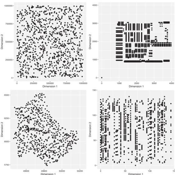
An example instance for each of the aforementioned four benchmark sets is de-picted in Figure 1. While instances from these four sets were already used in our initial work on algorithm selection for the TSP (Kotthoff et al., 2015), clustered instances were not considered then. These types of instances play an important role in many TSP ap-plications (e.g., vehicle routing), and we added two sets of clustered TSP instances to our overall benchmark.

Netgen Instances. This set of clustered instances, generated using the function

generateClusteredNetworkfrom the R-packagenetgen(Bossek, 2015), consists of mul-tiple instances for each combination of the number of citiesn∈ {500,1 000,1 500,2 000} and clustersnc∈ {2,5,10}.

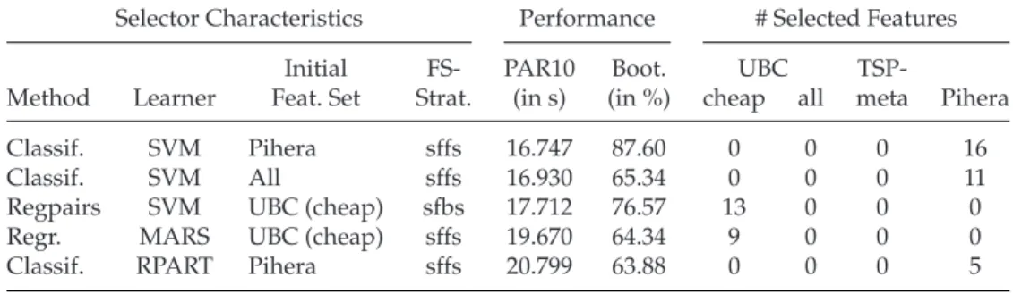
The instance generation process was introduced in Meisel et al. (2015) and works as follows: First a maximin Latin hypercube sample (LHS, McKay et al., 1979) of sizencis generated in two dimensions, that is,ncpoints are placed in the two-dimensional space maximising the minimal distance between design points. The space-filling property of LHS designs ensures that the cluster centres are evenly distributed across the space. Next, random points are sampled from a multivariate normal distribution per cluster using the cluster centres as the mean value vector and the distance to the nearest cluster centre as the variance in each dimension. The number of points is equally distributed across the clusters. Figure 2 shows two examples of such instances: one withnc=2 and n=50 (left) and one withnc=5 andn=250 (right).

Morphed Instances. In addition, we createdmorphedinstances, which combine prop-erties of RUE and clustered netgen instances, by using the morphing algorithm intro-duced by Mersmann et al. (2012) and improved by Meisel et al. (2015). It combines two instances with the same number of citiesnusing the following two-phase approach.

First, corresponding points in the two instances are matched by minimising the sum of Euclidean distances between matched points across all points through a linear programming formulation. Second, a convex combinationzij =α·xij+(1−α)·yij of the node coordinates of paired points xij andyij, wherei=1, . . . , nandj =1,2, de-termines the node coordinates in the corresponding morphed instancezij for a given morphing coefficient α∈[0,1]. Extreme values of α∈ {0,1}result in one of the input

Figure 1: Examples of TSP benchmark instances:1000-2(RUE; top left),d1291(drilling problem; TSPLIB; top right),lu980(980 cities in Luxembourg; National; bottom left), andpbd984(VLSI; bottom right).

instances, while other values of α generate intermediate instances, as illustrated in Figure 3.

The morphed instances used in our experiments were generated by applying the functionmorphInstances, available in the R packagenetgen, with morphing factorα= 0.5 to randomly selected instance pairs from the netgen and RUE sets.

Figure 2: Examples of netgen TSP instances with parametersnc=2 andn=50 (left), andnc=5 andn=250 (right) on a [0,100]×[0,100] grid. The white points indicate the locations of thenccluster centers (determined by means of maximin Latin hypercube sampling), and the black points indicate the actual cities to be visited.

Figure 3: Example of instance morphing of a 2-cluster instance into a RUE instance with n=100 nodes. A sequence of increasing morphing coefficientsα∈ {0,0.25,0.5,0.75,1} illustrates the transition between both instances.

3.4 Supervised Learning Methods for Algorithm Selection

A key aspect of this work is finding a suitable—that is, high-performance—algorithm selection model. We evaluated three supervised learning strategies, namely classifica-tion,regression, andpaired regression, with multiple machine learning techniques for each. In the classification approach, we label each instance with the best-performing TSP solver. In the regression approach, we predict the runtime for each solver on an instance separately and choose the solver with the lowest predicted runtime. The pairwise re-gression approach predicts the performance difference between two solvers for each pair of solvers. The solver with the best predicted performance difference to all other solvers is chosen. Further details regarding the setup and implementation of the three strategies can be found in Section 5.1.

Liaw and Wiener, 2002), and kernel-based support vector machines (ksvm, Karatzoglou et al., 2004) for each strategy. In addition, multivariate adaptive regression splines (mars, Leisch et al., 2016) were trained for the two regression approaches. Further details on MARS models can be found within Friedman (1991) or in the Appendix.

Each of the methods was used with its default settings, that is, without additional hyperparameter optimisation. Specifically, the random forests were built with 500 trees, using a uniform random sample of√p(classification) or max{p/3, 1}(regression / paired regression) of thepfeatures for each data set as candidates for each split point. The support vector machines used a Gaussian kernel with an a priori estimate of the inverse kernel width parameter, sigma, obtained using thesigest function from the

R-packagekernlab(Karatzoglou et al., 2004).

After training our algorithm selection systems based on these models, we assess their performance on a given TSP instance by determining the running time of the solver selected on that instance plus the running time required for computing the instance features used by the selector. To get reliable generalisation performance estimates on a given training set of instances, we use 10-fold cross-validation (further details will be given in Section 5).

3.5 Assessing the Significance of Performance Differences

In general, when comparing two TSP solvers,S₁andS₂(one or both of which may be algorithm selectors) on the same instance setI, we want to assess whether any observed difference in performance can be considered statistically significant. Here, performance is measured via the widely used PAR10 score (see, e.g., Bischl, Kerschke et al., 2016), which averages running time overI, counting runs that exceed the given cutoff time as ten times the cutoff. Our analysis addresses the question to which extent an observed difference in PAR10 scores depends on the particular given instance set,I. We therefore used bootstrap sampling to simulate drawing new instance sets from the distribution of problem instances that gave rise toI (Fawcett et al., 2017); following common practice, each sample was constructed using uniform random sampling with replacement and contains the same number of instances as I (Hastie et al., 2009). For each of theB= 10 000 bootstrap samplesI₁, . . . , IB thus obtained, we computed the PAR10 scores for S₁andS₂.

As a first measure of statistical stability, we determined the fraction of samples in whichS₁has a better (i.e., lower) PAR10 score thanS₂. The higher this fraction, the more confident we can be that a performance advantage ofS₁overS₂observed on benchmark setIalso holds for similar setsI(where technically, similarity means that both sets stem from the same underlying instance distribution).

To sharpen this analysis, we assessed the statistical significance of the performance difference betweenS₁ andS₂ onI by performing a one-sided Wilcoxon signed-rank test on the pairs of performance data (PAR10(S₁, Ib), PAR10(S2, Ib)) for b=1, . . . , B

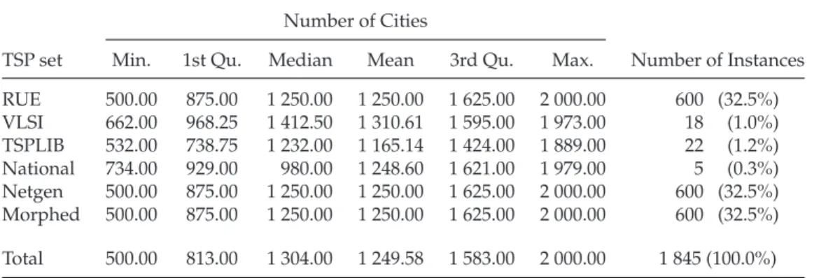
Table 1: Overview of the sizes and numbers of instances which were solved by at least one of the five algorithms and consist of 500 to 2 000 cities—per TSP set and in total. The problems are summarised by the minimum, first quartile (=25%-quantile), median, arithmetic mean, third quartile (=75%-quantile), and maximum.

Number of Cities

TSP set Min. 1st Qu. Median Mean 3rd Qu. Max. Number of Instances

RUE 500.00 875.00 1 250.00 1 250.00 1 625.00 2 000.00 600 (32.5%) VLSI 662.00 968.25 1 412.50 1 310.61 1 595.00 1 973.00 18 (1.0%) TSPLIB 532.00 738.75 1 232.00 1 165.14 1 424.00 1 889.00 22 (1.2%) National 734.00 929.00 980.00 1 248.60 1 621.00 1 979.00 5 (0.3%) Netgen 500.00 875.00 1 250.00 1 250.00 1 625.00 2 000.00 600 (32.5%) Morphed 500.00 875.00 1 250.00 1 250.00 1 625.00 2 000.00 600 (32.5%)

Total 500.00 813.00 1 304.00 1 249.58 1 583.00 2 000.00 1 845 (100.0%)

thanS₂ (say: 1 000 times). In this case,S₁would be much better thanS₂ according to PAR10 score and preferred in most practical situations, while the Wilcoxon signed-rank test onI (rather than bootstrap samples ofI) would indicate thatS₁ performs signifi-cantlyworsethanS₂, because used in this way, the test essentially ignores the magnitude of performance differences on the instancesi∈I.

For the analysis of our experimental results described in Section 6, we used R to gen-erate bootstrap samples and to carry out the Wilcoxon signed-rank test with a standard correction for ties (R Core Team, 2016).

4

Generating the Benchmark

First, we created a benchmark set of TSP instances based on the various instance sets introduced in Section 3.3. Using each of the instance generators, we produced an equal number of instances. In particular, for each of the instance sizes we considered, n∈ {500,1 000,1 500,2 000}, we generated 150 RUE instances, 50 netgen instances each for nc∈ {2,5,10}clusters, and 150 morphed instances obtained by combining those RUE and netgen instances with a morphing factor ofα=0.5. Thus, we obtained a grand total of 600 instances (4×150) each in our RUE, netgen and morphed sets. While the (mostly) real-world instances in the TSPLIB, National and VLSI sets have between 48 and 11 849 cities, to achieve better balance of instance sizes across our entire benchmark, we included only instances with 500 to 2 000 cities, resulting in 22 TSPLIB, 18 VLSI and 5 National instances, as shown in Table 1.

We note that our overall benchmark set is heavily biased towards the artificially generated RUE, netgen, and morphed instances, because we considered it important for the training of the machine learning models used in our algorithm selectors to have at our disposal a large set of TSP instances. We also note that the clustered and morphed instances, which jointly account for more than half of the overall set, show structure that is quite typical for many real-world TSP instances and known to be challenging for TSP solvers (see, e.g., Christofides, 1976; Solomon, 1987).

our benchmark set. As explained previously, each run was terminated as soon as an op-timal solution was found or after a cutoff time of 3 600 seconds; in the first case, the run was considered successful and in the second case, unsuccessful. We then recorded the median running time over these ten runs; if at least six of the ten runs were suc-cessful, the performance on that instance thus corresponds to the arithmetic mean of the fifth- and sixth-lowest running time. When fewer than six runs were successful, the performance on that instance was recorded as ten times the cutoff time, that is, 10 hours; this is the widely used PAR10 score (penalised average running time with penalisation factor 10).

Since the Pihera feature computation code is unable to handle instances with ATT edge weight type, we had to exclude the one instance in our set,att532from TSPLIB, in all experiments that included those edge weights.11 _{However, as the performance}

gap between the best (LKH) and worst (MAOS) solver on that instance is only 3.995 seconds, and we have 1 845 instances in total, the impact ofatt532on the PAR10 score of any solver or selector cannot exceed 3.995/1 845≈0.002 seconds.

Analysis of the feature values revealed that six of the Pihera features (nn3.Mdeg,

nn3.mindeg, nn3.sc.min, nn3.avg, nn5.avg, and nn7.avg), as well as the features

mst_depth_min(TSPmeta) andbc_no1s_q50 (UBC all) were constant across all 1 845 instances. As constant features do not provide any information to the machine learn-ing algorithms used for algorithm selection, these eight features were discarded. We also detected that two further Pihera features,nn5.Mdegandnn3.q3deg, were constant across 1 844 of our 1 845 instances. As explained in detail in Section 5, we evaluated our algorithm selectors using cross-validation (CV); we therefore discarded these two features as well, in order to avoid constant features within the training data of a single CV-fold. The detailed procedure for preprocessing the data is shown in Algorithm 1.

Note that we performed feature computation and solver runs on the same ma-chine, since we later take both into account to assess the performance of our algorithm selectors.

5

Experimental Setup

We trained the machine learning methods outlined in Section 3.4 to obtain algorithm se-lectors. With the exception of the scenarios in which we considered the Pihera features— and therefore had to discard TSPLIB instance att532 (as explained in the previous section)—all selectors were trained on the same set of 1 845 TSP instances, using the aggregated running times of the five TSP solvers that were introduced in Section 3.1, namely EAX, EAX+restart, LKH, LKH+restart, and MAOS. Following common prac-tice in machine learning, each selector was evaluated using 10-fold cross-validation.

Our selectors were either trained on one of the four feature sets from Section 3.2 or on the union of all four feature sets. Considering the high computational cost of these experiments and limitations of our computing resources, we did not explicitly consider combinations of two or three feature sets on top. However, as we performed feature selection based on the union of all feature sets (see Section 5.2), we implicitly also cover feature combinations that could stem from any combination of two or three feature sets. In the context of each of the selector construction approaches outlined in Section 3.4, we considered several machine learning procedures: classification and regression trees,

11_{We decided not to exclude the instance from our overall benchmark set, as it is one of the most}

support vector machines, and two variants of random forests.12 _{In addition, we also}

considered MARS models (see Section 3.4) in the two regression-based approaches, re-sulting in a total of 70 possible selectors (=5 feature sets×(4 classification+5 regression +5 paired regression machine learning procedures)).

5.1 Supervised Learning Strategies

Each of the three supervised learning strategies described below ultimately selects a TSP solver to use for each instance. Each of the selectors thus obtained is based on a specific feature set and consequently incurs a specific cost for determining the feature values for any given instance. These feature costs, as well as the running time of the selected TSP solver will then be averaged across all instances of the corresponding cross-validation fold, resulting in a PAR10 score per fold. These ten PAR10 scores are then again averaged across all ten folds, resulting in the algorithm selector’s PAR10 score.

Classification. The first strategy trains a machine learning model that predicts the best TSP solver for a given instance. The decision of whether a solver performed best on an instance is based on the aggregated running times. However, for 30 out of 1 845 instances (i.e., about 1.6% of our benchmark set), there was no clear best solver, that is, two or more

12_{While the trees, support vector machines, and MARS models are deterministic, the random forests}

solvers shared the lowest runtime. For those instances, we used the arithmetic mean of the unaggregated running times (for that instance) as a tie-breaking criterion.

Regression. While the classification approach does not consider the magnitude of the differences in running time, but solely relies on the best-performing solver on an in-stance, the regression approach directly models the running times of the solvers. This approach trains five models (one per solver) and afterwards selects the solver with the lowest predicted running time on the given TSP instance.

Paired Regression. The third approach models the differences in running time between pairs of solvers. That is, for each pair of solvers, we model the differences in running time, resulting in a total of ten models. We sum the running time differences per solver and choose the solver with the best total difference in running time. We note that this corresponds to a weighted voting scheme over pairs of solvers.

5.2 Feature Selection

We performed feature selection on each of the 70 algorithm selectors (i.e., on the un-derlying machine learning models) mentioned previously, using three different feature selection approaches, resulting in a total of 210 additional algorithm selectors. We used 10-fold cross-validation to assess the performance of our models, based on PAR10 scores (including the feature computation times). The computation of many features within each of the sets from Section 3.2 is deeply intertwined; therefore, if one or more fea-tures from a given set are selected, the associated feature computation time is always the same as for the entire set. During feature selection, ties between selectors with equal performance were broken uniformly at random.

Greedy Forward-Backward Selection. Our first feature selection approach,sffs (se-quential floating forward search), is a greedy forward-backward selection that starts with an empty set of features (Pudil et al., 1994); in our experiments, we used the vari-ant implemented in theR-packagemlr(Bischl, Lang et al., 2016). In each iteration, this procedure extends the given set F by the single feature not yet in F that gives the largest improvement in selector performance. After a feature has been added, the fea-ture whose exclusion leads to the largest improvement in performance is dropped and the next iteration begins, that is, a further feature is added. The process terminates when neither adding nor dropping any single feature leads to any improvement in selector performance.

Greedy Backward-Forward Selection. The second feature selection approach,sfbs (se-quential floating backward search, Pudil et al., 1994), works analogously tosffs, but in reverse. We used the variant implemented inmlr(Bischl, Lang et al., 2016), which works as follows: Starting with the full feature set, in each iteration, first the feature whose re-moval causes the largest improvement in performance is removed from the given set F, and then the feature, which is not yet inF, but leads to the largest improvement in performance overF, is added and the next iteration begins.

these so-calledparentsfrom the current population are used to create five new feature sets, the so-called offspring, using a mutation rate of 5% and crossover probability of 50%. Out of the resulting 15 feature sets—ten parents and five offspring—the ten best are chosen as the starting population for the next generation of the evolutionary process. We performed 100 generations of this genetic algorithm and chose the best individual from the final population as the feature set for our final selector.

5.3 Baseline Algorithms

As done in previous work on algorithm selection, we assess our selectors against two baselines: thevirtual best solverand thesingle best solver, to assess the performance of our algorithm selectors (Bischl, Kerschke et al., 2016).

Virtual Best Solver (VBS). This baseline, often also calledoracleorperfect selector, pro-vides the best possible performance on the given data by always choosing the best solver at no cost in addition to that incurred by running the selected solver. This idealised procedure provides an upper bound for the performance of any algorithm selector; be-cause of imperfect selection and feature computation cost, the performance of actual algorithm selectors usually falls short of that of the VBS.

Single-Best Solver (SBS). Our second baseline is given by the single solver available to any selector that shows the best aggregate performance on the given set of benchmark instances (here: the lowest PAR10 value). An algorithm selector is only useful if, taking feature costs into account, it performs better than the SBS. In principle, we could de-termine the SBS on our entire instance set or, for cross-validation, compute the SBS for each fold. On our data, this results in the same SBS.

6

Results

We now present a detailed performance analysis of the algorithm selectors we automat-ically constructed in our experiments.

6.1 Exploratory Data Analysis

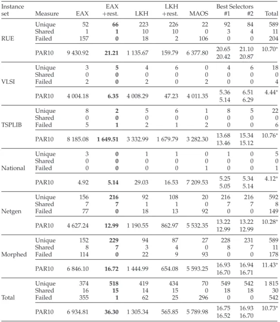
Table 2: Solver performance in terms of the number of instances that were solved best (relative to all other solvers); we additionally indicate for how many instances a given solver was the only one to achieve the best performance (unique), was tied with other solver for best performance (shared), or failed to find an optimal solution (failed), as well as running times (PAR10 scores, in seconds). The performances of our best two selec-tors are also shown, and the performance of the SBS (=EAX+restart) is printed inbold. The PAR10 scores of the selectors are shown including and excluding the cost of feature computation (top and bottom values, respectively). The PAR10 scores in the last col-umn (marked with∗) are those for the VBS. Note that all PAR10 scores within this table are computed without cross-validation, i.e., they are simply averaged across all the in-stances of the corresponding TSP set(s). Consequently, the performance values slightly differ from the values obtained from 10-fold CV shown in Table 3. Detailed interpreta-tions of the results shown below are given in Section 6.1.

Instance EAX LKH Best Selectors

set Measure EAX +rest. LKH +rest. MAOS #1 #2 Total

Unique 52 66 223 226 22 92 84 589

Shared 1 1 10 10 0 3 4 11

RUE Failed 157 0 18 2 106 0 0 204

20.65 21.10 10.70∗ PAR10 9 430.92 21.21 1 135.67 159.79 6 377.80

20.42 20.87

Unique 3 5 4 6 0 4 6 18

Shared 0 0 0 0 0 0 0 0

VLSI Failed 2 0 2 0 2 0 0 4

5.36 6.51 4.44∗ PAR10 4 004.18 6.35 4 008.29 47.23 4 011.35

5.14 6.29

Unique 8 2 5 6 1 8 5 22

Shared 0 0 0 0 0 0 0 0

TSPLIB Failed 5 1 2 1 2 0 0 6

13.68 15.34 10.76∗ PAR10 8 185.08 1 649.51 3 332.99 1 679.79 3 282.30

13.46 15.12

Unique 3 0 1 1 0 1 0 5

Shared 0 0 0 0 0 0 0 0

National Failed 0 0 0 0 1 0 0 1

5.25 5.34 4.12∗

PAR10 4.92 5.14 29.03 16.53 7 209.53

5.05 5.14

Unique 156 216 92 108 20 216 216 592

Shared 7 7 1 1 0 7 7 8

Netgen Failed 77 0 18 13 92 0 0 149

13.22 13.22 10.28∗ PAR10 4 627.24 12.99 1 190.55 862.97 5 532.35

12.99 12.99

Unique 152 229 94 87 27 228 231 589

Shared 8 7 3 4 0 8 7 11

Morphed Failed 114 0 22 9 93 0 0 178

16.93 16.94 11.43∗ PAR10 6 846.10 16.72 1 444.99 654.08 5 593.25

16.70 16.71

Unique 374 518 419 434 70 549 542 1 815

Shared 16 15 14 15 0 18 18 30

Total Failed 355 1 62 25 296 0 0 542

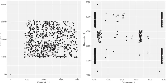
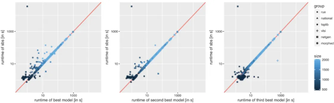
Figure 4: Scatterplots of the aggregated running times, shown on a log-scale, across our 1 845 benchmark instances. Left: Comparison of the virtual best solver (VBS) and the single best solver (SBS), that is, EAX+restart. Right: Comparison of the two best per-forming algorithms, LKH+restart and EAX+restart. While there is only one instance (d657 from TSPLIB, shown as a small dark square in the top left) that could not be solved by the SBS, LKH+restart failed to find the optimal tour for 25 instances (squares on the right margin of the plot).

A closer look at the running times required by each solver across our instance sets for finding optimal solutions reveals that, while LKH and LKH+restart clearly per-formed best on the largest number of RUE instances, their mean PAR10 scores (1 135.67 s and 159.79 s) are substantially worse than those of EAX+restart (21.21 s). The reason for this lies in the fact that LKH and LKH+restart often find an optimal tour quickly, but when they fail to do so, they take quite long, while EAX+restart shows much less ex-treme performance variation across different instances from the same benchmark set.

Table 2 also clearly indicates that the restart mechanisms integrated into EAX+ restart and LKH+restart achieve very substantial performance improvements com-pared to plain EAX and LKH. Interestingly, EAX benefits much more from restarting than LKH, as plain EAX shows the highest number of unsolved instances (355) and the worst PAR10 score of any of the solvers, whereas EAX+restart is the single best solver and fails to solve only a single instance across all of our benchmark sets. (We note that neither the benchmark sets nor the cutoff time were specifically chosen to achieve this level of performance.)

For LKH+restart, especially the clustered netgen and morphed instances turned out to be difficult to solve. On these instance sets, either variant of EAX ranked first more often than LKH+restart, and while EAX+restart always found an optimal tour within the given time budget, LKH+restart failed to solve 22 out of the 1200 instances.

Figure 5: Visualisation of two noteworthy TSPLIB instances. Left:d657, which was nei-ther solved by EAX, EAX+restart nor MAOS, whereas LKH and LKH+restart managed to find the optimal tour in less than a second. Right:p654, which was the only instance that EAX+restart solved in less than a second (0.76 s), while LKH (1.76 s), LKH+restart (2.47 s), and MAOS (4.41 s) needed much longer.

performance of the VBS provides an upper bound on the performance of any algorithm selector.)

Further evidence for this performance potential comes from the fact that the SBS needs more than one second for all but one instance (p654from TSPLIB, which is shown on the right of Figure 5), whereas the VBS finds an optimal tour in less than a second for 245 instances.

As can be seen in Figure 4 (right), LKH+restart and EAX+restart show qualitatively different performance characteristics: the running time of EAX+restart varies much less over instances of the same size. This is also reflected in the fact that the Spearman cor-relation coefficient between instance size and running time for LKH+restart is much lower (0.70) than for EAX+restart (0.91).

Instanced657from TSPLIB could not be solved by the SBS. Analyzing the perfor-mances of all five solvers on that instance, we found that neither EAX, nor EAX+restart or MAOS were able to solve this instance, whereas LKH and LKH+restart succeeded in less than one second. The instance is shown in Figure 5 (left); it resembles an RUE in-stance within the [1 000,4 000]×[1 000,3 000] box, with one additional city in the origin, (0,0). Interestingly, multiple runs of both EAX versions and of MAOS on the original instance failed, while all five solvers quickly succeeded on a customised replicate of that instance, which was created by sampling 656 cities random uniformly within the previously mentioned box-constraints extended by a city located in (0,0).

On the right side of Figure 5, we show the easiest instance for EAX+restart,p654

Table 3: Overview of the configuration, performance, and number of selected features (per feature set) of the five best performing algorithm selectors. All five selectors per-formed significantly better (p-value<10−16 _{in a Wilcoxon signed-rank test) than the}

single best solver (SBS), i.e., EAX+restart, whose PAR10 score was between 36.249 s (withoutatt532) and 36.362 s (withatt532). The table also lists how frequently each of the selectors performed better than the SBS, based on a comparison of 10 000 bootstrap samples.

Selector Characteristics Performance # Selected Features

Initial FS- PAR10 Boot. UBC

TSP-Method Learner Feat. Set Strat. (in s) (in %) cheap all meta Pihera

Classif. SVM Pihera sffs 16.747 87.60 0 0 0 16

Classif. SVM All sffs 16.930 65.34 0 0 0 11

Regpairs SVM UBC (cheap) sfbs 17.712 76.57 13 0 0 0

Regr. MARS UBC (cheap) sffs 19.670 64.34 9 0 0 0

Classif. RPART Pihera sffs 20.799 63.88 0 0 0 5

6.2 Comparison of Algorithm Selectors

Table 3 summarises the performance that was achieved by the best five algorithm se-lectors (according to their PAR10 scores) that we obtained from the experiment out-lined in Section 5. All of them perform significantly better than the single best solver (i.e., EAX+restart, with a PAR10 score of 36.3 s), closing most of the gap to the virtual best solver (with a PAR10 score of 10.7 s). We also note that only a small fraction of the available features are used by the best selectors, and that the feature selection step is crucial for obtaining high-performance selectors; none of the 70 selectors that used all features was able to beat the SBS. The best-performing selectors from Table 3 were more than 10 times better (in terms of PAR10) than the same selectors constructed with-out feature selection.

Our two best selectors are SVMs, which handle the algorithm selection problem as a classification problem. These two selectors are based on 16 and 11 Pihera features, respectively, but only three of the features are identical across both selectors. Other ap-proaches, for example, a regression-based MARS model, a paired-regression SVM, or a classification tree, also exceed the performance of the single best solver.

Noticeably, features from the TSPmeta and the full UBC feature sets—which on av-erage needed 9 to 12 s longer to compute (per instance) than features from the other two sets—were never selected by the best-performing selectors. Instead, these are ei-ther based on the cheap UBC or the Pihera feature set, but none of them uses features from both sets simultaneously, although the feature selection step in the construction of the second-best selector began with the union of all our feature sets. Overall, our results suggest that all feature sets are similarly informative, and if features from one of those sets are present, adding features from any of the other sets does not improve performance sufficiently to justify the increased cost.

Figure 6: Scatterplots of the running times, shown on a log-scale, across 1 844 benchmark problems (att532was excluded). Comparison of the the single best solver (SBS), that is, EAX+restart, and the best (left), second-best (middle), and third-best selector (right), respectively.

Comparing the PAR10 scores of our selectors and the individual TSP solvers we considered, our two best selectors always perform at least as well as any of the indi-vidual solvers (including the SBS) when ignoring the costs for the feature computation. The single best solver was only able to reach the performance of the best selector on the netgen instances, and the performance of the second-best selector on the netgen and National sets. For all other instance sets, our best two best selectors perform better than the SBS. When taking feature costs into account, our best selector beats the SBS on three of our six instance sets, and the second-best selector still beats the SBS on two instance sets.

We note that the SBS, EAX+restart, times out on TSPLIB instanced657. By choosing a different solver on that instance, all of our selectors avoid a substantial performance penalty amounting to almost 20 on the PAR10 score on the entire benchmark set. LKH and LKH+restart solve this instance in less than a second. As a result, while the PAR10 score for EAX+restart across the instances from TSPLIB was 1 649.51 s, our best selector achieved a score of 13.68 s.

Nevertheless, even when excluding this instance from the training set, our two best-performing selectors still performed statistically significantly better than the SBS: The PAR10 score of the SBS is 16.8 s, while the retrained versions of the top two selectors from Table 3 achieved PAR10 scores of 16.7 s and 16.4 s, respectively (including feature computation costs); these differences are small, but statistically significant according to a Wilcoxon signed-rank test atα=0.05.

Figure 6 illustrates the behaviour of our best three selectors in more detail. The instance at the top left isd657and all of our models correctly avoid selecting the SBS, EAX+restart, on this instance. For most instances however, the single best solver is the best choice; most points are very close to the diagonal, indicating that the selectors chose EAX+restart and that the costs for feature computation were negligible. The clouds of points on the upper left side of the diagonal show that especially the two best models improved over the SBS on many other instances as well.

7

Conclusion

performance complementarity—different solvers perform best on different TSP instances—and that this performance complementarity can be exploited by construct-ing per-instance algorithm selectors.

Our study presented here expands our own preliminary work (Kotthoff et al., 2015) substantially in scope and depth. Specifically, we considered an additional solver (MAOS), two additional types of TSP instances (netgen and morphed) and an addi-tional feature set (by Pihera and Musliu, 2014). More importantly, for the first time, we made extensive use of feature selection, which led to substantial performance im-provements in the selectors we were able to construct, as demonstrated using rigor-ous statistical tests. In addition to producing better TSP solver selectors, and hence an improvement in the state of the art in inexact TSP solving, we have also provided, for the first time, a detailed performance analysis of the best-performing inexact TSP solvers known previously.

In our exploratory data analysis, we confirmed that the restart mechanisms intro-duced by Dubois-Lacoste et al. (2015) substantially improve the performances of EAX and LKH. While EAX without the restart mechanism showed on average the worst per-formance of the five solvers we considered, EAX+restart was the single best solver. Nev-ertheless, performance also strongly depends on the TSP instances: although overall, EAX+restart showed the strongest performance on average, other solvers were found to perform better on many instances from our benchmark sets.

While we found multiple algorithm selectors with better performance than EAX+restart, the best two algorithm selectors are quite similar; both use support vector machines on a small subset of the feature set by Pihera and Musliu (2014), and each one of them improves the single best solver by a factor of two.

There are several directions for future work which we believe may lead to even better algorithm selectors. In our earlier work, we explored the use of so-called probing features, which are derived from partial runs of a TSP solver (Kotthoff et al., 2015). While we did not require such features here to produce very effective algorithm selectors, their use might lead to further performance improvements. Likewise, hyperparameter optimisation of the machine learning procedures at the heart of our selectors, though costly, might prove beneficial. Finally, based on our results presented here, we believe that a hybrid TSP solver that initially tries to find an optimal tour with a very fast solver (such as LKH) and then switches to EAX+restart might hold significant promise.

Acknowledgments

Holger Hoos acknowledges support from an NSERC Discovery Grant. Lars Kotthoff was supported by an NSERC Discovery Grant to Holger Hoos. Pascal Kerschke, Jakob Bossek, and Heike Trautmann acknowledge support from the European Research Cen-ter for Information Systems (ERCIS) and the DAAD PPP project No. 57314626.

References

Applegate, D. L., Bixby, R. E., Chvátal, V., and Cook, W. J. (2007).The traveling salesman problem: A computational study. Princeton: Princeton University Press.

Bischl, B., Kerschke, P., Kotthoff, L., Lindauer, T. M., Malitsky, Y., Fréchette, A., Hoos, H. H., Hutter, F., Leyton-Brown, K., Tierney, K., and Vanschoren, J. (2016). ASlib: A benchmark library for algorithm selection.Artificial Intelligence Journal, 237:41–58.

Bischl, B., Mersmann, O., Trautmann, H., and Preuss, M. (2012). Algorithm selection based on exploratory landscape analysis and cost-sensitive learning. InProceedings of the 14th Annual Conference on Genetic and Evolutionary Computation (GECCO), pp. 313–320.

Bossek, J. (2015).NetGen: Network Generator for Combinatorial Graph Problems. R-package version 1.0.

Christofides, N. (1976). The vehicle routing problem.Revue française d’automatique, d’informatique et de recherche opérationnelle (RAIRO). Recherche opérationnelle, 10(1):55–70.

Dubois-Lacoste, J., Hoos, H. H., and Stützle, T. (2015). On the empirical scaling behaviour of state-of-the-art local search algorithms for the Euclidean TSP. In Proceedings of the 17th Annual Conference on Genetic and Evolutionary Computation (GECCO), pp. 377– 384.

Eiben, Á. E., and Smith, J. E. (2015).Introduction to evolutionary computing. Berlin: Springer.

Fawcett, C., Hoos, H. H., Vallati, M., and Gerevini, A. E. (2017). What competition results really mean—Ranking solvers using statistical resampling. Under review.

Friedman, J. H. (1991). Multivariate adaptive regression splines.The Annals of Statistics, 1–67.

Fukunaga, A. S. (2000). Genetic algorithm portfolios. InProceedings of the IEEE Congress on Evolu-tionary Computation, vol. 2, pp. 1304–1311.

Gomes, C. P., and Selman, B. (2001). Algorithm portfolios.Artificial Intelligence Journal, 126(1-2):43– 62.

Hastie, T., Tibshirani, R., and Friedman, J. (2009).The elements of statistical learning: Data mining, inference, and prediction. 2nd ed. Berlin: Springer.

Helsgaun, K. (2000). An effective implementation of the Lin-Kernighan Traveling Salesman heuristic.European Journal of Operational Research, 126:106–130.

Helsgaun, K. (2009). General k-opt submoves for the Lin-Kernighan TSP heuristic.Mathematical Programming Computation, 1(2-3):119–163.

Hollander, M., Wolfe, D. A., and Chicken, E. (2013).Nonparametric statistical methods. 3rd ed. New York: John Wiley & Sons.

Huberman, B. A., Lukose, R. M., and Hogg, T. (1997). An economics approach to hard computa-tional problems.Science, 275(5296):51–54.

Hutter, F., Xu, L., Hoos, H. H., and Leyton-Brown, K. (2014). Algorithm runtime prediction: Meth-ods & evaluation.Artificial Intelligence Journal, 206:79–111.

Karatzoglou, A., Smola, A., Hornik, K., and Zeileis, A. (2004). Kernlab—An S4 package for kernel methods in R.Journal of Statistical Software, 11(9):1–20.

Kotthoff, L., Kerschke, P., Hoos, H. H., and Trautmann, H. (2015). Improving the state of the art in inexact TSP solving using per-instance algorithm selection. InProceedings of 9th International Conference on Learning and Intelligent Optimization, pp. 202–217. Lecture Notes in Computer Science, vol. 8994.

Kotthoff, L. (2014). Algorithm selection for combinatorial search problems: A survey.AI Magazine, 35(3):48–60.

Leisch, F., Hornik, K., and Ripley, B. D. (2016).MDA: Mixture and Flexible Discriminant Analysis. R-package version 0.4-9.

Malitsky, Y., Sabharwal, A., Samulowitz, H., and Sellmann, M. (2013). Algorithm portfolios based on cost-sensitive hierarchical clustering. InProceedings of the 23rd International Joint Conference on Artificial Intelligence, pp. 608–614.

McKay, M. D., Beckman, R. J., and Conover, W. J. (1979). A comparison of three methods for select-ing values of input variables in the analysis of output from a computer code.Technometrics, 21(2):239–245.

Meisel, S., Grimme, C., Bossek, J., Wölck, M., Rudolph, G., and Trautmann, H. (2015). Evaluation of a multi-objective EA on benchmark instances for dynamic routing of a vehicle. In Pro-ceedings of the 17th Annual Conference on Genetic and Evolutionary Computation (GECCO), pp. 425–432.

Mersmann, O., Bischl, B., Bossek, J., Trautmann, H., Wagner, M., and Neumann, F. (2012). Local search and the Traveling Salesman Problem: A feature-based characterization of problem hardness. InProceedings of 6th International Conference on Learning and Intelligent Optimization, pp. 115–129. Lecture Notes in Computer Science, vol. 7219.

Mersmann, O., Bischl, B., Trautmann, H., Preuss, M., Weihs, C., and Rudolph, G. (2011). Ex-ploratory landscape analysis. InProceedings of the 13th Annual Conference on Genetic and Evo-lutionary Computation (GECCO), pp. 829–836.

Mersmann, O., Bischl, B., Trautmann, H., Wagner, M., Bossek, J., and Neumann, F. (2013). A novel feature-based approach to characterize algorithm performance for the Traveling Salesperson Problem.Annals of Mathematics and Artificial Intelligence, 69:151–182.

Mu, Z., Dubois-Lacoste, J., Hoos, H. H., and Stützle, T. (2017). On the empirical scaling of running time for finding optimal solutions to the TSP. Under review.

Nagata, Y., and Kobayashi, S. (1997). Edge assembly crossover: A high-power genetic algorithm for the Travelling Salesman Problem. InProceedings of the 7th International Conference on Ge-netic Algorithms, pp. 450–457.

Nagata, Y., and Kobayashi, S. (2013). A powerful genetic algorithm using edge assembly crossover for the Traveling Salesman Problem.INFORMS Journal on Computing, 25(2):346– 363.

O’Mahony, E., Hebrard, E., Holland, A., Nugent, C., and O’Sullivan, B. (2008). Using case-based reasoning in an algorithm portfolio for constraint solving. In Proceedings of the 19th Irish Conference on Artificial Intelligence and Cognitive Science, pp. 133– 142.

Pihera, J., and Musliu, N. (2014). Application of machine learning to algorithm selection for TSP. InProceedings of the IEEE 26th International Conference on Tools with Artificial Intelligence,pp. 47–54.

Pudil, P., Novoviˇcová, J., and Kittler, J. (1994). Floating search methods in feature selection.Pattern Recognition Letters, 15(11):1119–1125.

R Core Team (2016).R: A language and environment for statistical computing. Vienna: R Foundation for Statistical Computing.

Rice, J. R. (1976). The algorithm selection problem.Advances in Computers, 15:65–118.

Sander, J., Ester, M., Kriegel, H.-P., and Xu, X. (1998). Density-based clustering in spatial databases: The algorithm GDBSCAN and its applications.Data Mining and Knowledge Dis-covery, 2(2):169–194.

Smith-Miles, K., and van Hemert, J. (2011). Discovering the suitability of optimisation algorithms by learning from evolved instances.Annals of Mathematics and Artificial Intelligence, 61(2):87– 104.

Solomon, M. M. (1987). Algorithms for the vehicle routing and scheduling problems with time window constraints.International Journal of Operations Research, 35(2):254–265.

Therneau, T., Atkinson, B., and Ripley, B. (2015).RPART: Recursive Partitioning and Regression Trees. R-package version 4.1-10.

Xie, X.-F., and Liu, J. (2009). Multiagent optimization system for solving the Traveling Sales-man Problem (TSP).IEEE Transactions on Systems, Man, and Cybernetics, Part B: Cybernetics, 39(2):489–502.

Xu, L., Hutter, F., Hoos, H. H., and Leyton-Brown, K. (2008). SATzilla: Portfolio-based algorithm selection for SAT.Journal of Artificial Intelligence Resesearch, 32:565–606.

Xu, L., Hutter, F., Hoos, H. H., and Leyton-Brown, K. (2011). Hydra-MIP: Automated algorithm configuration and selection for mixed integer programming. InProceedings of the 18th RCRA Workshop on Experimental Evaluation of Algorithms for Solving Problems with Combinatorial Ex-plosion at the International Joint Conference on Artificial Intelligence, pp. 16–30.

Xu, L., Hutter, F., Hoos, H. H., and Leyton-Brown, K. (2012). Evaluating component solver contri-butions to portfolio-based algorithm selectors. InProceedings of the 15th International Confer-ence on Theory and Applications of Satisfiability Testing, pp. 228–241. Lecture Notes in Computer Science, vol. 7317.

Appendix

While recursive partitioning and regression trees, random forests and kernel-based sup-port vector machines are all popular machine learning approaches,multivariate adaptive regression splines(MARS, Friedman, 1991) are less prominent. We still considered MARS, because we observed promising performance in preliminary experiments; furthermore, the underlying idea is simple and appealing.

A MARS model is a combination of piecewise polynomial functions, so-called splines. More formally, the model can be written as a function

ˆ

f(z)=c₀+ K

k=1

ck·bk(z)

with model coefficientsc₀, . . . , cK, basis functionsb1(z), . . . , bK(z) and ap-dimensional input vectorz=(z₁, . . . , zp)T. The basis functionsbk, fork=1, . . . , K, stem from a set

H= {(zj −x1j)q₊,(x1j −zj)q₊, . . . ,(zj −xNj)q₊,(xNj−zj)q₊}j₌1,...,p

of so-calledhinge functions. Each of them is a polynomial (of orderq) of the difference be-tween thej-th input variablezj and a realization of this variable from the training data, x₁j, . . . , xNj, the so-calledknots. Furthermore, the hinge function limits the polynomial to non-negative values, i.e., (zj −xij)

q