The impact of strong gravitational lensing on observed Lyman-break
galaxy numbers at 4
≤
z
≤
8 in the GOODS and the XDF blank fields
R. L. Barone-Nugent,
1‹J. S. B. Wyithe,
1M. Trenti,
1,2T. Treu,
3P. Oesch,
4R. Bouwens,
5G. D. Illingworth
6and K. B. Schmidt
31School of Physics, University of Melbourne, Parkville, VIC 3010, Australia
2Kavli Institute for Cosmology and Institute of Astronomy, University of Cambridge, Cambridge CB2 1TN, UK 3Department of Physics, University of California, Santa Barbara, CA 93106-9530, USA
4Department of Astronomy, Yale University, New Haven, CT 06511, USA 5Leiden Observatory, Leiden University, NL-2300 RA Leiden, the Netherlands 6UCO/Lick Observatory, University of California, Santa Cruz, CA 95064, USA
Accepted 2015 March 23. Received 2015 March 3; in original form 2014 December 18
A B S T R A C T
Detections of Lyman-break galaxies (LBGs) at high-redshift are affected by gravitational lensing induced by foreground deflectors not only in galaxy clusters, but also in blank fields. We quantify the impact of strong magnification in the samples ofB435,V606,i775andz850&Y105
dropouts (4z8) observed in the eXtreme Deep Field (XDF) and the Cosmic Assembly Near-infrared Deep Extragalactic Legacy Survey (CANDELS) fields by investigating the proximity of dropouts to foreground objects. We find that∼6 per cent of brightz∼7 LBGs (mH160 <26) have been strongly lensed (μ >2) by foreground objects. This fraction decreases from∼3.5 per cent atz∼6 to∼1.5 per cent atz∼4. Since the observed fraction of strongly lensed LBGs is a function of the shape of the luminosity function (LF), it can be used to derive Schechter parameters,αandM, independently from galaxy number counts. Our magnification bias analysis yields Schechter-function parameters in close agreement with those determined from galaxy counts albeit with larger uncertainties. Extrapolation of our analysis toz8 suggests that surveys withJWST,WFIRSTandEuclidshould find excess LBGs at the bright end, over an intrinsic exponential cutoff. Finally, we highlight how the magnification bias measurement near the XDF detection limit can be used to probe the population of galaxies beyond this limit. Preliminary results suggest that the magnification bias atMUV ∼ −18 is
weaker than expected ifα−1.7 extends well below the current detection limits. This could imply a flattening of the LF atMUV −16.5. However, selection effects and completeness
estimates are difficult to quantify precisely. Thus, we do not rule out a steep LF extending to
MUV−15.
Key words: gravitational lensing: strong – galaxies: high-redshift – galaxies: luminosity
function, mass function – cosmology: observations.
1 I N T R O D U C T I O N
Surveys of Lyman-break galaxies (LBGs) during the epoch of reionization aim to make a census of high-redshift galaxies and to estimate the available ionizing photon budget for reionization (Khochfar et al.2007; Bouwens et al.2008,2011,2014; Castellano et al. 2010; Bradley et al. 2012; Finkelstein et al. 2012, 2014; Oesch et al. 2012; McLure et al. 2013; Robertson et al.2013; Schenker et al.2013; Schmidt et al.2014). These surveys, however,
E-mail:robertbn@student.unimelb.edu.au
may provide an increasingly skewed view of the early Universe as redshift increases. The observations are complicated by gravita-tional lensing (Wyithe et al.2011), which affects the observed lumi-nosities and surface density of high-redshift LBGs. Along random lines of sight, the probability of significant magnification and mul-tiple images from gravitational lensing is∼0.5 per cent (Barkana & Loeb2000; Comerford, Haiman & Schaye2002; Wyithe et al.
2011). Furthermore, high-redshift luminosity functions (LFs) have been shown to have very steep faint-end slopes (α ∼ −1.6 at z∼4 toα∼ −2.0 atz∼8, although the uncertainties are large, e.g. Bouwens et al.2014; Schmidt et al.2014), which results in a bias leading to an enhanced probability of gravitational lensing over
Magnification bias is expected to significantly skew the observed bright end of the LF at very high redshifts (see fig. 3 in Wyithe et al.2011). The effect is intriguing in light of thez∼7 LF, which has been observed to both agree with the exponential cutoff in the Schechter parametrization (Bouwens et al.2014), and also to de-cline less steeply than a Schechter function (Bowler et al.2014). Previous studies of high-redshift galaxies have argued that gravita-tional lensing has not significantly affected their LFs (McLure et al.
2006), while others have made slight corrections in the observed luminosities of LBGs due to gravitational lensing (Bowler et al.
2014). However, even though the sample sizes analysed in recent studies are large, the numbers of bright galaxies, where the mag-nification bias effects will be most apparent, remain small. Thus observational verification of any changes to the slope at the bright end remains to be determined.
Identifying and confirming individual cases of strong gravita-tional lensing of LBGs atz4 is made difficult due to sources appearing faint and small. Elongation in the observed LBG due to lensing is difficult to detect due to their small observed size compared with the resolution of the telescope. Secondary images are very difficult to observe, as they will be less magnified than the primary image, and hence be extremely faint (Barone-Nugent et al.2013). Secondary images will also appear closer to the deflec-tor than the primary image, making it more difficult to disentangle them from the deflector galaxy light than the primary image. Wyithe et al. (2011) calculated the probability of detecting a secondary im-age to be≈10 per cent, where the bright image of a galaxy is 1 mag above the survey limit.
In this paper, we adopt a statistical approach to detect gravita-tional lensing of high-redshift galaxies using the largest samples of LBGs at 4≤z≤8 (Bouwens et al.2014). We assess the likeli-hood of lensing for each individual LBG in homogenous samples atz∼ 4,z ∼ 5,z∼ 6 and z∼ 7–8 in order to infer the total expected lensed fraction at a range of flux limits. In Section 2, we describe the data used in our analysis. In Section 3, we derive the Faber–Jackson relation (FJR; Faber & Jackson1976) of fore-ground galaxies that we will use in our analysis. Section 4 describes our method of prescribing a likelihood of lensing to each LBG. Section 5 describes our lensing results and in Section 6, we assess the magnification bias and the consequences for the LF beyond cur-rent survey limits. In Section 7, we assess the observational effects of magnification bias on the LF and in Section 8, we present the strong lensing likelihoods of existingz∼9–10 LBGs. In Section 9, we conclude. We refer to theHST F435W,F606W,F775W,F850LP,
F105W,F125WandF160Wbands asB435,V606,i775,z850,Y105,J125 andH160. Throughout this paper, we useM=0.3,=0.7 and
LBGs ‘drop out’ in theB435,V606,i775,z850andY105for LBGs at
z∼4,z∼5,z∼6,z∼7 andz∼8, respectively. The catalogues include 5867, 2108, 691, 455 and 155 LBG candidates atz∼4, z∼5,z∼6,z∼7 andz∼8, respectively.
We use the 3D-HST photometric catalogue of the CANDELS area (Brammer et al.2012; Skelton et al.2014) in order to model foreground objects as potential gravitational lenses. The 3D-HST survey covers all of the CANDELS fields, with spectroscopy com-piled from the literature. We utilize the spectroscopic redshifts of foreground objects when available, and otherwise rely on pho-tometric redshifts obtained using EAZY (Brammer, van Dokkum & Coppi2008) which are based on deep multiband observations (Taniguchi et al. 2007; Barmby et al. 2008; Erben et al. 2009; Grogin et al.2011; Koekemoer et al.2011; Whitaker et al.2011; Bielby et al.2012; Brammer et al.2012; McCracken et al.2012; Ashby et al.2013).
We calibrate a redshift-dependent Faber–Jackson relation (Faber & Jackson1976) in Section 3 using early-type galaxy data from Treu et al. (2005), Auger et al. (2009) and Newman et al. (2010). The galaxies in these samples have published spectroscopic redshifts, velocity dispersions and rest-frameB-band magnitudes.
3 T H E FA B E R – J AC K S O N R E L AT I O N
There exists a spatial correlation between bright, high-zLBGs and bright foreground objects (see Appendix A). Spatial correlations between source LBGs and foreground objects suggests that mag-nification bias is detectable in current surveys. In order to quantify its extent, foreground objects need to be modelled as gravitational lenses.
The key parameter determining the efficiency of an early-type galaxy as a gravitational lens is its velocity dispersion (Turner, Ostriker & Gott1984). We estimate the velocity dispersion of each galaxy in the CANDELS field from its photometry by calibrating a redshift-dependent Faber–Jackson relation (FJR; Faber & Jackson
1976). The FJR relates the luminosity of an object to its velocity dispersion. We include a redshift evolution term to account for the evolution of the mass-to-light ratio with increasing redshift, so the FJR can be expressed as
LB =mσγ(1+z)β, (1)
whereLBis theB-band luminosity, σ is the stellar velocity dis-persion andzis the redshift. The FJR can be expressed linearly as
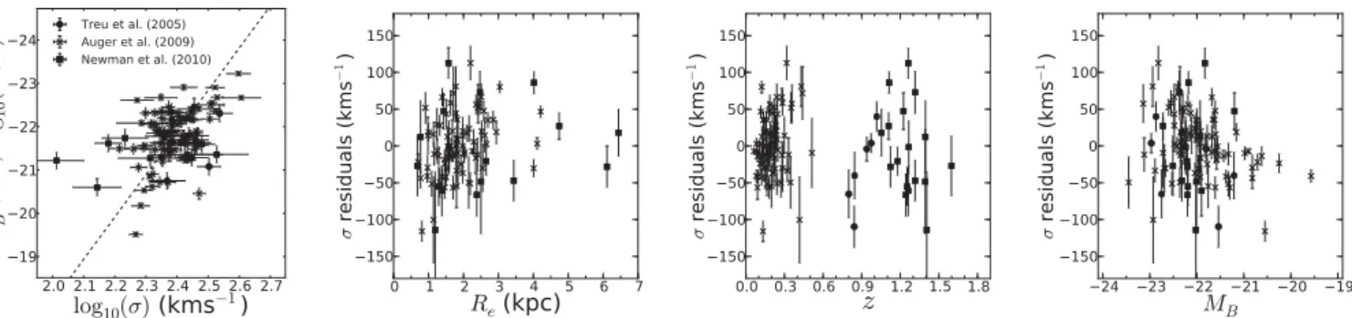
Figure 1. Left: the FJR that we derive (dashed) projected along thez-axis and the galaxies in the three samples of Treu et al. (2005), Auger et al. (2009) and Newman et al. (2010). We find no systematic biases in the FJR we derive. Centre left: the residuals of the velocity dispersions of the galaxies in the Auger et al. (2009) and Newman et al. (2010) samples as a function of effective radius. Centre right: the residuals of the velocity dispersions of the galaxies in the three samples as a function of redshift. The scatter in the residuals atz >0.6 agrees with the scatter in the residuals atz <0.6 within the uncertainties. Right: the residuals of the velocity dispersions as a function of theB-band magnitude.
wherea= −2.5γ,x=log10 σ
200 km s−1,b= −2.5β,y=log10(1+z), c= −2.5 log10(m) andMB= −2.5 log10(LB). We calibrate the FJR using galaxies with spectroscopic redshifts and velocity dispersions from Treu et al. (2005), Auger et al. (2009) and Newman et al. (2010), which span 0< z <1.6. We determine the values ofa,b
andcby minimizing theχ2, given by
χ2=
n
i=0
(MBi −axi−byi−c)2
2
MBi +a2x2i+b
22
yi+
2 int
, (3)
whereMB,x,yare the uncertainties in the data andintis the intrinsic scatter. To avoid degeneracies, we fix the slope to beγ =3.9, in line with previous studies (Hyde & Bernardi2009a; J¨onsson et al.
2010).
We find best-fitting parameters ofm= 2.3± 0.2×10⁸ and
β=0.7±0.3. The errors onmandβare not independent, so the uncertainty in the inferred velocity dispersion due to their uncer-tainty is∼10 km s−1, and will not significantly affect the inferred strongly lensed fraction. The FJR is plotted in the left-hand panel of Fig. 1, and the residuals are plotted as a function of effective radius, Re, redshift,z, andB-band magnitude,MBare plotted in the centre-left, centre-right and right-hand panels, respectively. The uncertainty in the FJR is dominated by the intrinsic scatter, which is 46 km s−1in the direction of velocity dispersion. There are no systematic biases in the residuals with respect toMB,zor theRe. The scatter in the residuals for galaxies atz >0.6 is consistent with galaxies atz <0.6, with no evidence of redshift-dependent scatter in our FJR.
The resultant FJR is consistent withB-band FJRs found from weak lensing analyses of Type Ia supernovae presented by J¨onsson et al. (2010), Kleinheinrich et al. (2006) and Hoekstra, Yee & Gladders (2004). As a check of our FJR, we compare it with the
i-band FJR (which may be less prone to dust-extinction) presented by Bernardi et al. (2003) for all objects in GOODS. We find very close agreement betweenσas inferred from thei-band FJR with ourB-band FJR. For low-redshift objects, the scatter in the resid-uals between the two methods is 2 km s−1. For all objects out to
z=2, the scatter in the residuals between the two FJRs is 9 km s−1. This may be partially due to the Bernardi et al. (2003) FJR being calibrated atz∼0, and not taking into account redshift evolution. There are no systematic biases in the residuals between these two FJRs as a function ofz,MBorRe.
We compare our FJR with estimates of velocity dispersions using the stellar mass estimates of galaxies in our calibration sample using the relation between stellar mass and velocity dispersion presented
by Hyde & Bernardi (2009b). We find the scatter in the residuals of velocity dispersion estimates using this method to be very sim-ilar (in fact, slightly larger) than those found using our FJR. This suggests that using stellar mass information rather thanLBwill not significantly reduce the scatter in our velocity dispersion estimates.
4 A S S E S S I N G T H E S T R O N G L E N S I N G L I K E L I H O O D O F L B G S
To quantify the strongly lensed fraction of LBGs, we model every foreground object in the field as a gravitational lens. Using photo-metric information of all foreground objects, we ask the following question for each LBG: What is the likelihood of this LBG being gravitationally lensed with magnificationμ >2 given its position relative to nearby (in projection) foreground objects? We disregard deflector–LBG pairs with a separation ofθsep>5.0 arcsec, which is much larger than the Einstein radius of typical deflectors. While the choice of maximum separation of 5.0 arcsec is somewhat arbitrary, we show in Section 5.2 that 5.0 arcsec is a reasonable choice. For each foreground object within 5.0 arcsec of the LBG, we use the following process.
(i) Model the foreground object using a singular isothermal sphere (SIS) density profile.
(ii) Calculate the velocity dispersion that the foreground object requires for it to produce an image at the observed position of the LBG with a magnification ofμ = 2, denoted byσ,req. For an SIS,μ=2 marks the beginning of the strong lensing regime. The required velocity dispersion depends on the LBG–deflector separation, LBG redshift and deflector redshift.
(iii) Calculate the likelihood that the foreground object has a ve-locity dispersion greater than or equal toσ,req. This is the likelihood of strong lensing for that deflector–LBG pair.
(iv) Weight the likelihood of lensing by the inverse of the de-tection completeness at the separation between the LBG and the nearby foreground object.
The final step accounts for reduced sensitivity to faint LBGs nearby bright foregrounds. We explain this process further in Section 4.1.
To calculateσ,reqwe find the Einstein radius,θER, required for
μ=2 using the expression for the magnification of the image in an observed configuration
μ= |θsep|
|θsep| −θER
Figure 2. Examples of possibly lensed LBGs in the four samples. All cutouts are of theJ125images, are 10.0×10.0 arcsec and are shown on the same contrast scale (except for the top-left cutout, which contains two very bright foreground galaxies). The LBGs are circled in red and the deflectors are labelled by their spectroscopic/photometric redshifts. Each LBG is labelled with itsH160magnitude, and its likelihood of being strongly lensed (top-left corner). The LBG shown in the bottom-left panel is the brightest LBG in thez∼7 sample.
whereμis the magnification, andθsep is the observed separation between the source image and the deflector. We can then find the velocity dispersion corresponding toμ=2 using the expression for the Einstein radius of an SIS
θER=4π σ
c
2D LS
DS
, (5)
whereσis the stellar velocity dispersion,DSis the angular diameter distance to the source andDLSis the angular diameter distance from the lens to the source.
For each LBG–foreground object pair, the likelihood of strong lensing of the LBG by the deflector is equal to the likelihood that the deflector has a velocity dispersion aboveσ,req, which is given by
L = 1
2erfc
σ,req−σ,inf
√ 2FJR
, (6)
whereσ,inf is the velocity dispersion inferred from photometry (using the FJR), and FJR is the intrinsic scatter in the velocity dispersion of the FJR.
In the event that there are multiple potential deflectors within 5.0 arcsec of the source, we treat them independently and calculate the probability that at least one is lensing the source byμ≥2. For
ndeflectors, this is
L =1−
n
j=1
(1−Lj). (7)
We show a subset of the sample consisting of some of the highest-likelihood lenses in Fig.2. We describe these systems further in Section 5.1.
4.1 Accounting for sensitivity variations
Faint LBG samples have a reduced completeness compared to bright ones. This alone would not affect our inference of the lensed frac-tion, because the completeness would change the numerator and the denominator by the same factor at fixed magnitude. However, we note that there may be a further reduced sensitivity to detect-ing faint LBGs around bright objects, which will affect potentially lensed LBGs differently to those isolated in the field. This effect could cause our measured strongly lensed fraction to be artificially low.
We weight all LBGs that appear close in projection to bright foreground objects by the inverse of their relative detection proba-bility in order to account for reduced sensitivity around foreground objects. To do this, we run completeness simulations around all foreground objects which are either
(i) assessed as having a greater than 1 per cent chance of lensing a nearby LBG, or,
(ii) brighter thanmr=24 mag and within 2.5 arcsec of an LBG.
We run source recovery simulations in order to determine complete-ness as a function of radius around each foreground meeting either of the above criteria. The source recovery simulations are run for LBGs1at the redshift and of the magnitude corresponding to that of the nearby LBG. The completeness of a source LBG,sc, becomes unaffected by typical foregrounds at a separation of around 1.5– 2.0 arcsec. The weight,wc, we apply to each LBG is defined as
the inverse of the completeness,wc≡1/sc. We apply a maximum weighting ofwc=10 to any LBG.
We find that weighting the lensed fraction in this way has a minimal effect on the bright end of the observed lensed fraction. However, the relative completeness of faint galaxies near to bright foreground galaxies is, as expected, lower than for the brighter LBGs.
4.2 Uncertainty checks
The typical uncertainty in the photometric redshifts of foreground sources derived in the 3D-HST catalogues arez∼0.1–0.2, so the uncertainty in the magnification is dominated by the intrinsic uncertainty in the FJR. Furthermore, the uncertainty inMBdue to photometric redshift errors (via the distance modulus) is partially self-regulating as the inferred velocity dispersion is a decaying func-tion of redshift, while inferred rest-frame luminosity is an increasing function. We find that of the 40z∼7 LBGs that have a likelihood of lensing of≥10 per cent, the deflector of only one has a photomet-ric redshift with less than an 80 per cent chance of residing within z=0.2. None of the deflectors ofz∼4–6 LBGs with a likelihood of lensing of≥10 per cent have photometric redshifts with less than an 80 per cent chance of residing withinz=0.2. The uncertainty in source redshift (z∼0.35) is negligible as the angular diameter distance is a relatively flat function at high redshift.
There is a possible Eddington bias stemming from uncertainties in the photometry and the shape of the LF atz∼1, which could bias the inference ofσfrom theB-band luminosity. We find that (L ± δL) only varies by 2–5 per cent from(L) for galaxies brighter than ∼M atz = 1 in the field. Therefore, the number density of bright galaxies does not change significantly within the photometric uncertainties, and the Eddington bias is negligible.
We note that a limitation of this analysis is that it assumes all deflectors to be SISs. Singular isothermal ellipsoids (SIEs) may be a more realistic parametrization of potential deflectors (see Keeton 2001, for ellipsoidal density parametrizations). However, SIEs do complicate the calculation significantly (Kormann, Schnei-der & Bartelmann1994; Huterer, Keeton & Ma2005). The median ellipticity for all objects in the CANDELS fields is=0.21, with 83 per cent having an ellipticity of <0.4. In the case of low deflec-tor ellipticity ( 0.2), the change in the magnification estimate is≈10 per cent along both the major (+10 per cent) and minor (−10 per cent) axes. For larger ellipticities ( 0.4), the magnifi-cation estimate becomes≈20 per cent lower for an image located along the minor axis, and a factor of 2 higher for images along the major axis. Using an elliptical deflector model for the system shown in the bottom, centre-left panel of Fig.2, which includes a deflector with large ellipticity (=0.48), we estimate the magnification to beμ 1.6, as compared with the SIS estimation ofμ 1.8. The LBG in the bottom-right panel of Fig.2, which is near a deflector with ellipticity=0.33, has a magnification ofμ 1.6 in the SIS model, which becomesμ 1.9 using an ellipsoidal model.
Similarly, the lensing cross-section (the strong lensing area in the image plane owing to a deflector) of an SIE is the same as the optical depth of an SIS with a higher order term (Kormann et al. 1994). The area of sky covered by the Einstein radius of an SIE is only ≈5 per cent larger than the area of sky covered by an SIS for reasonable ellipticities ( 0.4). Therefore, our calculations of the optical depth in Section 6 are not significantly affected by the SIS assumption. These calculations are consistent with previous studies of the effect of ellipticity on the strong lensing optical depth and magnification, such as Huterer et al. (2005) who
noted that aside from image multiplicities, introducing shear and ellipticity has surprisingly little effect. Hence, using an SIE deflector will not qualitatively change either our strongly lensed fraction or magnification bias results.
5 T H E S T R O N G LY L E N S E D F R AC T I O N
The method of prescribing a likelihood of strong lensing described in Section 4 was applied to each LBG in the samples atz∼4,z∼ 5,z∼6 andz∼7–8. The 455z850dropouts and 155Y105dropouts were combined to create a statistically significant sample with a mean redshift of z=7.2. The number of strongly lensed LBGs brighter than a theoretical survey limit,mlim, is assessed for each of the samples. For thei775, andz850&Y105samples, we assess the lensed fraction brighter thanmlim=26, 27, 28, 29 and 30 mag in H160. We includemlim=25 mag for theV606sample andmlim=24 and 25 for theB435sample, asMappears brighter for these samples. The strongly lensed fraction is not affected by the differing depth of the CANDELS fields and the XDF.
The cumulative lensed fraction at each of these flux limits is the ratio of the expected number of strongly lensed LBGs (the sum of all lens likelihoods) brighter than the flux limit and the total number of LBGs appearing brighter than the flux limit. However, the cumulative lensed fraction depends on the total completeness of the combined sample. To account for incompleteness in number counts, we use the LF of Bouwens et al. (2014). The cumulative lensed fraction atz∼4,z∼5,z∼6 andz∼7 is shown in the left-hand panel of Fig.3. The right-hand panel of Fig.3shows the observed magnification bias (see Section 6). When inferring properties of the LF (Sections 6.1 and 6.2) we use the observed lensed fraction in each bin without LF-correction so as to not presuppose the nature of the LF.
The trend to a larger fraction of strongly lensed galaxies for brighter flux limits is reasonably smooth, monotonic and observed in each of the four independent samples. The amplitude at all flux limits steadily increases fromz∼4 toz∼7 (although the error bars are large), which is expected as the faint-end slope steepens and the strong lensing optical depth increases at higher redshift. The excess probability of gravitational lensing of bright galaxies is detected at high significance in each of the samples. The lensed fraction of LBGs brighter thanmH160=26 is∼6 per cent atz∼7 and∼3.5 per cent atz∼6, although the uncertainty is large due to the rarity of bright objects at high redshift. Atz∼5, the lensed fraction at the same flux limit is∼3.5 per cent and atz∼4 the lensed fraction is ∼1.5 per cent.
We also assess the lensed fraction at brighter flux limits for the z∼4 andz∼5 samples. We find that the lensed fraction continues to rise, as expected. Atz∼5,∼5 per cent of LBGs brighter than
m=25 are strongly lensed, and atz∼4,∼4.5 per cent of LBGs brighter thanm=24 are lensed.
The errors are calculated using bootstrap resampling. The boot-strap sample is drawn from the entire sample with replacement
N=104times. Each time, each LBG is considered either ‘lensed’ or ‘not lensed’ randomly according to its likelihood of having been lensed. The lens fraction is recalculated for all limiting fluxes. The error bars represent the 1σ limits of the resultant distributions.
5.1 Examples of likely lensed systems
Figure 3. Left: the lensed fraction of background LBGs as a function of flux limit for thez850andY105-dropout samples (blue),i775-dropouts (red, offset by m+0.1),V606-dropouts (green, offset bym+0.2) andB435-dropouts (yellow, offset bym+0.3). The observed lensed fraction decreases monotonically with decreasing redshift for flux limits ofmlim=26, 27, 28 and 30. The analytic strong lensing optical depths,τ, (strongly lensed fraction of random lines of sight) for each source redshift are plotted as dashed lines in the same colours as the observed lensed fractions (see Section 6). Right: the observed magnification bias at each redshift overlaid as a function ofM−Mlim(see Section 6). TheB435sample contains the brightest measurements with respect toM(1 mag brighter), followed by theV606sample, thez850&Y105sample and thei775sample. The bias is defined as the ratio of the solid and dashed lines in the left-hand panel. We show the bias at each redshift individually in Fig.5. For an LF without strong evolution inα, which is approximately observed from 4< z <7, the bias is not expected to evolve. A roughly constant bias is observed at all values ofM−Mlimfor the four independent LBG samples from 4< z <7.
importance to future surveys. We note that the three brightestzand
Y-dropouts in the entire sample are each deemed to have a likelihood of lensing of>10 per cent. The brightest LBG in thez∼7 sample is shown in the bottom-left panel of Fig.2. All cutouts are shown at the same contrast scale, except for thez∼4 lens candidate (top left), which is in proximity to two very bright foreground galaxies, both withMB∼ −23.5, one of which is spectroscopically confirmed atz=0.8. All cutouts are 10.0 arcsec on each side. In each case, the deflector candidate is labelled with its spectroscopic or photometric redshift and the LBG is labelled with itsH160magnitude.
The cutouts highlight the difficulty in locating secondary images in the event the LBG has been strongly lensed. A secondary im-age will appear closer to the foreground galaxy than the primary (circled) image, and is likely to also appear much fainter than the primary image.
5.2 Deflector properties
We present the distribution of the image–deflector separations, de-flector redshifts and dede-flectorB-band absolute magnitudes in this section. The number of lensed sources is weighted by the likelihood of lensing for each image–deflector configuration.
The top row of Fig.4shows the distribution of lens rest-frame
B-band magnitudes for each of the four independent LBG samples. The peak of the distribution occurs aroundMB∼ −22 for each of the samples.
The middle row of Fig. 4 shows the distribution of image– deflector separations for each of the LBG samples. The normal-ized cumulative fractions are shown as dashed lines. We observe an approximate increase in the peak of the separation distribution as redshift increases (from∼1.0 arcsec atz∼4 to∼2.0 arcsec at z∼7), consistent with the expectation that higher redshift sources have larger deflection angles.
The bottom row of Fig.4 shows the distribution of deflector redshifts. The normalized cumulative fractions are shown as dashed lines. We observe an increase in the peak of the deflector redshift
distribution fromz∼ 4 sources, where the deflector distribution peaks aroundz∼1, to thez∼7 sources, where the peak occurs aroundz∼2. This evolution is consistent with the expectation that lenses are most likely to be found at around half of the angular diameter distance to the source.
6 M AG N I F I C AT I O N B I A S
The total magnification bias of a flux-limited sample,B(L > Llim), is the ratio of the fraction of strongly lensed galaxies and the frac-tion of strongly lensed random lines of sight, defined as thestrong lensing optical depth,τ (e.g. Wyithe et al.2011). We generate a catalogue of 50 000 random source positions in the GOODS fields and use the method of assessing the lensed fraction presented above in Section 4 to determine the fraction of the source plane that will be strongly lensed. Based on our FJR, we assess the strong lensing optical depth for sources atz∼4,z∼5,z∼6 andz∼7.2 to be τ=0.41, 0.54, 0.65 and 0.75 per cent. The values found are broadly consistent with theoretical predictions of the strong lensing optical depths at these redshifts (Barkana & Loeb2000; Wyithe et al.2011; Mason et al.2015). Due to the large number of foregrounds in the CANDELS fields, the relative statistical uncertainty onτ is only ∼4 per cent in all samples, and hence negligible in our bias calcu-lations. We find consistent values for the optical depth if we apply a reasonable upper limit of∼350 km s−1on the inferred velocity dispersion of foreground galaxies. We find that our method of de-termining the optical depth returns values in close agreement with those in Mason et al. (2015) when we adopt their method of infer-ring velocity dispersions using stellar mass estimates.2The optical depths are plotted as dashed lines in Fig.3.
The bias is therefore the observed magnified fraction divided by the optical depth (the solid lines divided by the dashed lines in
Figure 4. The lensing-likelihood-weighted distributions (solid) and cumulative distributions (dashed) of deflector properties. These distributions illustrate the diversity and evolution of the deflector population in the four samples analysed. Top row: the distribution ofB-band absolute magnitudes of the deflectors for the four LBG samples. Middle row: the distribution of image–deflector separations for the four LBG samples. Bottom row: the distribution of redshifts of the deflectors for the four LBG samples.
Fig.3). The observed total bias for each of the samples at a range of flux limits is plotted in the right-hand panel of Fig.3and the top row of Fig.5. The bias reaches values of∼10 at bright magnitudes and high redshifts, but near the survey flux limit has values lower than expected for a LF that remains steep well beyond survey limits. We calculate the observed magnification bias in each bin (as opposed to the total magnification bias for all galaxies brighter than a flux limit). The results are plotted in the bottom row of Fig.5.
For an LF with weak (or no) redshift evolution of theαparameter, the magnification bias as a function ofM −Mlim is expected to remain approximately constant with redshift. To highlight that this trend exists in the data, we plot the observed magnification bias at each redshift on the same axes in the right-hand panel of Fig.3. While α evolves from∼−1.6 to ∼−2.0 fromz ∼ 4 toz ∼ 8, the statistical uncertainties in our measurements are larger than the change in bias from this evolution.
For a given LF,(L), the magnification bias can be predicted analytically (Turner et al.1984) at luminosityL, by
B(L)=
μmax
μmin
dμ
μ ddPμ(L/μ)
(L) , (8)
where the 1/μ factor accounts for the stretching of (L/μ)dμ with magnification, and ddPμis the magnification distribution for the brighter image in a strongly lensed system, given for an SIS by
dP dμ =
2
(μ−1)3 for 2< μ <∞
0 forμ <2 . (9)
We assume(L) to be the Schechter LF. The analytic magnification bias for all galaxies in a flux-limited sample is
B(L > Llim)= μmax
μmin dμ
∞
LlimdL
dP
dμ(L/μ)
∞
LlimdL(L)
, (10)
where the factor of 1/μis no longer included because we are now integrating over luminosity, and hence the luminosity limits are also stretched byμin the numerator.
Results for our bias estimates given the Schechter LF parame-ters in Bouwens et al. (2014) and theoretical curves are plotted in Fig.5. The top row compares the theoretical bias of all galaxies in a flux-limited sample with our measurements of the observed bias for all galaxies in a flux-limited sample. The bottom row shows the theoretical bias of galaxies at a fixed luminosity with our mea-surements of the observed bias in each magnitude bin. Theoretical values for bias are calculated using previously derived LF param-eters αand M (Bouwens et al.2014) and a range of values at which the LF deviates from a steep faint-end slope. We find close agreement between the observed shape and amplitude of the magni-fication bias and the theoretical function in each of the independent samples.
Figure 5. Top row: the observed total magnification bias of all galaxies brighter than a flux limitM−Mlim(solid) compared with the theoretical magnification bias for the LFs (described by equation 10) from Bouwens et al. (2014) with a range of magnitudes at which the LF flattens (α∼ −1), denoted byMturn. The cumulative lensed fraction is corrected for incompleteness according to the LF of Bouwens et al. (2014). Bottom row: the observed magnification bias in each bin plotted at the mean luminosity of the bin. At faint magnitudes in each sample of LBGs, the bias falls below the value expected from a faint-end slope continuing well beyond the survey limit, indicating a possible deviation from a steep faint-end slope of the LF, although they agree with theory within their error bars. For an LF with a steep faint-end slope continuing well beyond the flux limit, the bias flattens to a value ofB∼2–3 (depending onα). The measurements of bias at a fixed luminosity do not need to be corrected for incompleteness.
6.1 The faint-end slope beyond current flux limits
Magnification bias results from magnification of intrinsically faint sources below an observed flux limit into an observed sample, hence quantifying the degree of magnification bias offers an opportu-nity to investigate the behaviour of the LF beyond current survey limits.
To illustrate, we begin with a toy model in which there is a minimum luminosity for galaxies ofLmin, below which there are no galaxies, and a power-law slope ofα= −2.0 forL>Lmin. In this toy model, a sharp cutoff in the LF at a value ofLminyields a bias of
B(L > Llim)= ⎧ ⎨ ⎩
3− 2
Llim/Lmin−1 forLlim>2Lmin
1 forLmin< Llim<2Lmin
.
(11)
This implies the total bias of a flux-limited sample reaches unity approximately 1 mag brighter thanLmin. We observe a hint of the possibility of this occurring in the four samples presented in this paper, as seen in the top row of Fig.5. The bottom row of Fig.5
also highlights this behaviour in our samples.
Rather than a sharp cutoff in the LF, we consider a more re-alistic model with an LF that flattens (α2 = −1) after some lu-minosity,Lturn. We attempt to constrain Lturn by finding an LF that will reproduce the observed magnification bias in the
bot-tom row of Fig. 5. Using a broken Schechter function of the form
(L)dL=
⎧ ⎪ ⎪ ⎪ ⎨ ⎪ ⎪ ⎪ ⎩
,1
L L
α1
exp
− L L
dL
L forL≥Lturn
,2
L L
α2
exp
− L L
dL
L forL < Lturn,
(12)
withα2= −1 (i.e. a flat LF beyondLturn), we fit the bias calculated from equation (8) to the data withLturn,α1andMas free parameters.
We include priors on the values ofα1 and M, from the LFs of Bouwens et al. (2014). Fig.6shows the constrains found for the minimum luminosity from our analysis fitting to two subsets of our measurements. The dashed black line in Fig.6shows the probability distribution function (PDF) when fittingMturnto the observed bias of only LBGs brighter thanm=29, and the solid line shows the PDF when fitting to LBGs brighter thanm=30 (approximately the 5σ limit in the XDF). The PDFs are normalized such that the probability ofMturn<−12 is unity. We find preferred values ofMturnto peak around the current observational limits in each of the independent samples from 4< z <7. The sample atz∼6 peaks at a magnitude brighter than flux limits, which can be ruled out observationally. We also calculate the likelihoods with an additional prior enforcing
Mturnto occur below the magnitude that the steep faint-end slope has been observed to extend to. These are plotted in red in Fig.6
Figure 6. The inferred value ofMturnusing the magnification bias measurements of all galaxies brighter thanm<30 (solid) and all galaxies brighter than m<29 (dashed). The bias measurements which we fit to are shown in the bottom row of Fig.5. In black we plot the likelihoods with a prior onαandMfrom Bouwens et al. (2014, see table 4 therein for values). The red curves show the estimated likelihoods including an additional requirement that the minimum magnitude is fainter than the magnitude to which current observations confirm a steep faint-end slope. We find approximately consistent preferred values of Mturnin each of the four samples, but with varying amplitudes. For LBGs brighter thanm=30 (approximately the 5σXDF limit, solid line), we find a preferred value ofMturnaround the observational limits in each sample. However, a value ofMturn>−16 is not excluded. For only LBGs brighter thanm=29 (dashed line), we find no constraint onMturnin any of the samples. This is expected, because to constrainMturnwe need to consider galaxies within∼1–2 mag ofMturn. The curves are normalized such that the probability ofMturn<−12 is unity.
inference ofMturnoccurring close to current flux limits is marginal and does not rule out a faint-end slope extending well beyond current flux limits, or a flattening for a few magnitudes followed by an upturn.
We find that the constraint disappears whenMturnis fitted to only brighter (m< 29) galaxies. We extend this test by recalculating our results by omitting XDF LBGs entirely from the analysis to investigate whether the observed magnification bias will always approach unity near the flux limit due to selection effects. When we perform this test, we find the magnification bias of galaxies in the GOODS-North and GOODS-South is completely consistent with that of the full sample, rather than approaching unity near the flux limit.
It is important to note that the magnification bias is only observed to drop below its expected value close to the current flux limits where selection effects become significant. While we have taken care to account for the decreased sensitivity to very faint sources, there still exists the possibility that we have missed a significant fraction of gravitationally lensed LBGs at very faint magnitudes. Furthermore, if the interloper fraction at very faint fluxes is high, the lensed fraction will be underestimated, causing a spurious inference ofMturn.
The possibility of a flattening of the LF atMturn ∼ −16.5 at
z ∼7 is consistent with observations of LBGs down toMUV ∼
−15.5 of magnifiedz∼7 LBGs using Frontier Fields cluster Abell 2744 (Atek et al. 2015; Ishigaki et al.2015). Fig. 7 shows the Bouwens et al. (2014) and Atek et al. (2015) data with the best-fitting broken Schecter function (α2= −1). We find that a broken Schechter function represents the data very well, and offers an independent constraint onMturn. The data favour a value ofMturn∼
−16.5, consistent withMturninferred from our magnification bias results. However, as is the case with our magnification bias analysis, this inference is based on a single data point.
Further to this study atz∼7, there exist measurements of the UV LF ofz∼2 LBGs down toMUV∼ −13 (Alavi et al.2014). While a single Schechter function favours a steep slope extending toMUV∼ −13 atz∼2, the shape of the LF at the faint end may be more complicated than this simple parametrization. In fact, the data also seem to suggest a flattening of the population density between
Figure 7. Thez∼7 LF data from Bouwens et al. (2014, blue circles) and Atek et al. (2015, black squares) with the best-fitting broken Schechter LF (dashed) and single Schechter LF (dotted). The solid line shows the likelihood ofMturn given the two data sets. We find a favoured flattening magnitude atMUV∼ −16.5, consistent with our magnification bias mea-surements.
−17 MUV −15, before a steeper upturn from−15 MUV
−13 (see Alavi et al.2014, fig. 7). This more complicated LF would produce a reduced magnification bias (B(L>Llim)∼1) of
z∼2 LBGs near a flux limit ofMUV ∼ −17.5, which is on the edge of current survey limits in blank fields (Reddy & Steidel2009; Hathi et al.2010; Oesch et al.2010; Sawicki2012). Additionally, a flattening, and potentially a rise in the LF atMUV−15 would not be inconsistent with the inference from GRB host galaxies studies (Tanvir et al. 2012; Trenti et al. 2012; Trenti, Perna & Tacchella2013). In fact, these studies only constrain the presence of an abundant population of galaxies below the XDF detection limit, but not the shape of the galaxy LF, which theyassumeto be Schechter-like. Interestingly, theoretical models that are based on a double population of faint galaxies have been proposed in the context of hydrogen reionization (e.g. see Alvarez, Finlator & Trenti
from Bouwens et al. (2014, red) and Finkelstein et al. (2014, yellow) are shown for comparison. We find close agreement between the two methods atz∼4 andz∼5, while the constraints atz∼6 andz∼7 from lensing are weaker due to the larger error bars on the magnification bias measurements.
6.2 Deriving Schechter parameters from lensing
A very interesting application of this analysis is that Schechter function parameters αand M can be derived directly from the magnification bias. This method is completely independent of the standard procedure using number counts of galaxies, and therefore could be combined to produce improved constraints.
The magnification bias at a fixed luminosity can be predicted using equation (8), and is a function ofαandM. By fitting the predicted bias of LBGs at a fixed flux to our measured bias in each flux bin (which is shown in the bottom row of Fig.5, and is not the LF-corrected cumulative fraction), we can constrainαandM.3 This does not rely on any prior knowledge of the LF. Becauseα andMare much more sensitive to the bias of bright galaxies than that of faint galaxies, and we see a possible deviation from a single Schechter function at faint magnitudes, we exclude the two faintest bins (29<m<30, and 28<m<29) from the fit.4Fig.8shows the constraints on the LF from the observed magnification bias alone along with the constraints from number counts of the same samples. The measurements of the bias atz∼4 andz∼5 do an excellent job of constraining the LF. At higher redshift, as the samples become smaller and the random errors grow, we cannot constrain the LF as effectively. However, we find that our observations are consistent with the UV LFs presented by Bouwens et al. (2014). This also provides an internal consistency check of our analysis.
6.3 Contaminant discussion
We check for bias arising from the selection of LBGs. There may be an enhancement and reddening of LBG candidates observed around bright, red foreground galaxies due to photometric scatter, causing an increased fraction of interlopers around such foreground objects and providing a false lensing signal among bright candidates. To determine if this may affect our results, we check if an enhanced interloper fraction around bright foregrounds is found in lower red-shift LBG samples for which there exists spectroscopic follow-up.
3We fit the theoretical bias at the mean magnitude of the LBGs in each magnitude bin to the observed bias in that bin withαand M as free parameters.
4In fact, fitting the data including the two faintest bins with an extra free parameter,Mturn, and marginalizing over this parameter gives the same result.
We combine catalogues with spectroscopically confirmed LBGs and photometrically selected LBGs which were identified as inter-lopers from 3< z <6 using observations reported by Vanzella et al. (2009), Reddy et al. (2006), Malhotra et al. (2005) and Steidel et al. (2003). We compare the fraction of interlopers for LBGs within 5.0 arcsec of bright, red foreground galaxies (mr<−22 mag) with the fraction of interlopers in the total sample. In both cases, we find the interloper fraction to be∼8 per cent, with 2 of 25 LBGs around bright foreground galaxies identified as interlopers, and 21 of 252 of the entire sample. This indicates that the alignment between bright LBGs and massive foreground galaxies is not likely due to selec-tion bias. The large enhancement in false identificaselec-tions required to mimic the observed magnification bias of∼10 for bright galaxies is clearly inconsistent with the spectroscopic data.
7 M AG N I F I C AT I O N B I A S A N D T H E L F
The effect of magnification bias on determining the LF is an impor-tant consideration when making a census of galaxies in the epoch of reionization (Wyithe et al.2011; Mason et al.2015). In this section, we show the effect that the lensed fraction reported in this paper has on the observed LF.
The observed LF of LBGs is the convolution between the intrinsic LF,(L), and the magnification distribution of an SIS,ddPμ, weighted by the strong lensing optical depth,τ. This results in an observed LF,obs(L), with a power-law tail at the bright end with a slope of−3 (the slope of the magnification distribution of an SIS). We assess the effect of gravitational lensing on the LF by following the method presented by Wyithe et al. (2011), where it is modelled by considering the optical depth,τ, the mean magnification of multiply imaged sources for an SIS,μmult =4, and the demagnification of unlensed sources (to conserve total flux on the cosmic sphere), μdemag =(1− μmultτ)/(1−τ). The observed LF is then given by
obs(L)=(1−τ) 1 μdemag
(L/μdemag)
+τ
∞
0 dμ1
μ
dPm,1 dμ +
dPm,2 dμ
(L/μ), (13)
where dPm,2
dμ =2/(μ+1)
3for 0< μ <∞is the second image’s
magnification probability distribution, and dPm,1
Figure 9. The effect of magnification bias on the bright end of the LFs
z∼4,z∼5,z∼6,z∼7,z∼8 andz∼10 (LBGs become monotonically more abundant with decreasing redshift atMUV≤ −22). The observed LFs are shown as solid lines, and the intrinsic LFs as dashed lines. The LF measurements from Bouwens et al. (2014) and Bowler et al. (2014) are plotted as circles and diamonds, respectively. Atz∼7,z∼8 andz∼10, observations are close to probing the bright end where gravitational lensing becomes a significant effect, but not bright enough for it to be manifested in the observed LF.
presented in Section 6, and calculate the optical depth atz=6.8, z =7.9 and z= 10.4 to beτ = 0.72 , 0.80 and 0.94 per cent, respectively.
We begin by assuming that the observed LF is not affected by gravitational lensing and hence represent the intrinsic LFs. We plot these intrinsic LFs (Bouwens et al.2014), the inferred observed LF and observations (Bouwens et al.2014; Bowler et al.2014) at z∼4,z∼5,z∼6,z∼7,z∼8 andz∼10 in Fig.9(dashed lines). Fig.9also shows the biased LFs, illustrating the luminosity at which gravitational lensing becomes important. This also illustrates the assumption that current LF measurements are not significantly affected by magnification bias is sound.
The effect of magnification bias is not significant at the faint end of the LF. At around 2 mag fainter thanM, the excess observed abundance of LBGs is of the order of 0.5 per cent for all of the samples, which is significantly smaller than the observational errors in the abundances at these magnitudes.
We note that even the brightest Bowler et al. (2014) and Bouwens et al. (2014) measurements are not bright enough to probe the affected region of the LF. However, the effect magnification bias will have on surveys atz8 is obvious from the solid lines forz∼ 8 andz∼10 where the observed LF will display a break from the intrinsic LF aroundMUV−22.5.
Not plotted in Fig.9are extrapolated LFs atz >10. Wyithe et al. (2011) showed that ifMdrops sharply at high redshifts, surveys of the depth of the XDF withJWSTwill observe galaxies atz >10 in the affected region of the LF.
8 A N A LY S I S O F C U R R E N T J125- D R O P O U T S
In Section 7, we presented the effect that magnification bias has on the observed LF. Fig.9highlights that while magnification bias is not a significant effect in current surveys out toz∼8, the af-fected region of thez∼ 10 LF begins at aroundMUV ∼ −22.5. We investigated the four unusually brightz∼10J125-dropouts
pre-sented by Oesch et al. (2014) to search for evidence of lensing. This point is discussed in Oesch et al. (2014), where they find there is the possibility of a modest amount of lensing in two of the four dropouts. By applying the technique employed in this paper, we assign likelihoods of lensing to the fourz∼9–10 LBGs.
As noted by Oesch et al. (2014), two of the LBGs are not close in projection to any foreground objects (GN-z10-3 and GN-z9-1 in the notation of Oesch et al.2014), while the other two do have projected neighbours (GN-z10-1 and GN-z10-2). GN-z10-1 is 1.2 arcsec from a foreground galaxy atzphot=1.6 withMB= −20.1 (using photometry from the 3D-HST catalogue). Oesch et al. (2014) infer a photometric redshift ofz=1.8). Using our redshift-evolving FJR, this corresponds to a stellar velocity dispersion of 140 km s−1. The required stellar velocity dispersion for strong-lensing in this case is 198 km s−1, giving this LBG a likelihood of lensing ofL = 0.12. GN-z10-2 is 2.9 arcsec from a bright galaxy atzspec=1.02 withMB= −20.7. This corresponds to an inferred stellar velocity dispersion of 214 km s−1. The required stellar velocity dispersion for strong lensing is 279 km s−1, giving a likelihood of lensing ofL =0.1. While the statistics are too small to draw any firm conclusions, this average observed lensed fraction of∼6 per cent for the four galaxies is consistent with a lensed fraction of LBGs brighter thanMof∼10 per cent.
9 S U M M A RY
We have estimated the likelihood of strong gravitational lensing of LBGs in the XDF and GOODS atz∼ 4,z ∼ 5,z∼ 6 and z∼7. We used a calibrated FJR to estimate the lensing potential of all foreground objects in the fields. The result is a measurement of significant magnification bias in current high-redshift samples of LBGs. Our analysis allows us to draw the following conclusions.
(i) Approximately 6 per cent of LBGs atz∼7 brighter thanM
(mH160∼26 mag) are expected to have been strongly gravitationally lensed withμ >2.
(ii) The observed strongly lensed fraction of LBGs at all values of mH160 falls monotonically from z ∼ 7 to z ∼ 4, which can be explained by the expected evolution in the optical depth with redshift, and alsoMappearing brighter at lower redshift.
(iii) By evaluating the optical depth in our lensing framework, we calculate the magnification bias in each sample as a function of
M−Mlim, and find that the results agree at each redshift and are well described by theoretical predictions.
(iv) Extrapolation of our analysis leads to expectations for an increased fraction of strongly lensed galaxies atz8, consistent with Wyithe et al. (2011).
(v) The magnification bias of the faintest LBGs in the sample suggests there may be a flattening of the faint-end slope below current detections limits (MUV−16.5). However, this result relies on LBG detections at low S/N in the XDF, and the constraints are weak. We present this result tentatively, with deeper data needed to better understand the population of faint high-zgalaxies.
(vi) Assessing the magnification bias as a function of luminosity offers an independent method of determining Schechter parameters αandM. The results from this method are consistent with those found by fitting the LF based on number counts.
Alavi A. et al., 2014, ApJ, 780, 143
Alvarez M. A., Finlator K., Trenti M., 2012, ApJ, 759, L38 Ashby M. et al., 2013, ApJ, 769, 80
Atek H. et al., 2015, ApJ, 800, 18
Auger M., Treu T., Bolton A., Gavazzi R., Koopmans L., Marshall P., Bundy K., Moustakas L., 2009, ApJ, 705, 1099
Barkana R., Loeb A., 2000, ApJ, 531, 613
Barmby P., Huang J.-S., Ashby M., Eisenhardt P., Fazio G., Willner S., Wright E., 2008, ApJS, 177, 431
Barone-Nugent R., Wyithe J., Trenti M., Treu T., Oesch P., Bradley L., Schmidt K., 2013, preprint (arXiv:1303.6109)
Bernardi M. et al., 2003, AJ, 125, 1849 Bielby R. et al., 2012, A&A, 545, A23
Bouwens R. J., Illingworth G. D., Franx M., Ford H., 2008, ApJ, 686, 230 Bouwens R. et al., 2011, ApJ, 737, 90
Bouwens R. et al., 2014, preprint (arXiv:1403.4295) Bowler R. et al., 2014, MNRAS, 440, 2810 Bradley L. et al., 2012, ApJ, 760, 108
Brammer G. B., van Dokkum P. G., Coppi P., 2008, ApJ, 686, 1503 Brammer G. B. et al., 2012, ApJS, 200, 13
Calvi V., Pizzella A., Stiavelli M., Morelli L., Corsini E., Dalla Bont`a E., Bradley L., Koekemoer A., 2013, MNRAS, 432, 3474
Castellano M. et al., 2010, A&A, 524, A28
Comerford J. M., Haiman Z., Schaye J., 2002, ApJ, 580, 63 Erben T. et al., 2009, A&A, 493, 1197
Faber S., Jackson R. E., 1976, ApJ, 204, 668 Finkelstein S. L. et al., 2012, ApJ, 758, 93
Finkelstein S. L. et al., 2014, preprint (arXiv:1410.5439) Grogin N. A. et al., 2011, ApJS, 197, 35
Hathi N. et al., 2010, ApJ, 720, 1708
Hoekstra H., Yee H. K., Gladders M. D., 2004, ApJ, 606, 67 Huterer D., Keeton C. R., Ma C.-P., 2005, ApJ, 624, 34 Hyde J. B., Bernardi M., 2009a, MNRAS, 394, 1978 Hyde J. B., Bernardi M., 2009b, MNRAS, 396, 1171 Illingworth G. et al., 2013, ApJS, 209, 6
Ishigaki M., Kawamata R., Ouchi M., Oguri M., Shimasaku K., Ono Y., 2015, ApJ, 799, 12
J¨onsson J., Dahl´en T., Hook I., Goobar A., M¨ortsell E., 2010, MNRAS, 402, 526
Keeton C. R., 2001, preprint (astro-ph/0102341)
Khochfar S., Silk J., Windhorst R., Ryan R., Jr, 2007, ApJ, 668, L115 Kleinheinrich M. et al., 2006, A&A, 455, 441
Koekemoer A. M. et al., 2011, ApJS, 197, 36
Kormann R., Schneider P., Bartelmann M., 1994, A&A, 284, 285 McCracken H. et al., 2012, A&A, 544, A156
McLure R. et al., 2006, MNRAS, 372, 357 McLure R. et al., 2013, MNRAS, stt627 Malhotra S. et al., 2005, ApJ, 626, 666
Mashian N., Loeb A., 2013, J. Cosmol. Astropart. Phys., 12, 017 Mason C. et al., 2015, preprint (arXiv:1502.03795)
Trenti M., Perna R., Levesque E. M., Shull J. M., Stocke J. T., 2012, ApJ, 749, L38
Trenti M., Perna R., Tacchella S., 2013, ApJ, 773, L22 Treu T. et al., 2005, ApJ, 633, 174
Turner E. L., Ostriker J. P., Gott J. R., III, 1984, ApJ, 284, 1 Vanzella E. et al., 2009, ApJ, 695, 1163
Whitaker K. E. et al., 2011, ApJ, 735, 86 Windhorst R. A. et al., 2011, ApJS, 193, 27
Wyithe J. S. B., Yan H., Windhorst R. A., Mao S., 2011, Nature, 469, 181 Yue B., Ferrara A., Vanzella E., Salvaterra R., 2014, MNRAS, 443, L20
A P P E N D I X A : S PAT I A L C O R R E L AT I O N S B E T W E E N B R I G H T F O R E G R O U N D S A N D L B G S
In this appendix, we present the manifestation of magnification bias in spatial correlations between bright foreground objects and bright LBGs, which illustrates the effect without relying on the FJR.
Source galaxies that have been magnified through gravitational lensing are necessarily located in close proximity to massive fore-ground objects. For the lensed fractions presented in Section 5, we expect there to be an excess density of bright LBGs around bright foreground objects over the average field density. As the lensed fraction decreases with decreasing luminosity, the excess proba-bility around bright deflectors should also decrease. Similarly, the clustering around the more massive, brighter deflectors should be stronger than around less massive, fainter deflectors.
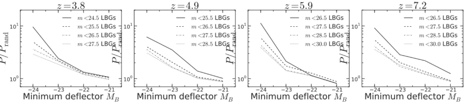
We compute the excess probability of finding an LBG brighter thanm=30, 28.5, 27.5 and 26.5 atz=7.2 within 5.0 arcsec of de-flectors brighter than someMB. We choose 5.0 arcsec as our limit as this is approximately the image–deflector separation beyond which strong lensing is unlikely. This is confirmed by the distribution of separations shown in Fig.4. We also present the spatial correlations for the lower redshift samples. Atz=5.9, we examine the same flux limits, atz=4.9 we replacemlim=30 withmlim=25.5 and atz=3.8 we replacemlim=28.5 withmlim=24.5. The results are plotted in Fig.A1.
We find a large enhancement in the probability of finding bright LBGs nearby bright deflectors. As we consider fainter LBGs, the excess probability decreases monotonically in all of the samples. There exists a considerable excess of LBGs around foregrounds with
MB<−23 atz≥4, even for flux limits well beyondM; however,
Figure A1. The excess probability of finding an LBG brighter than various flux limits within 5.0 arcsec of deflectors brighter thanMBatz <2. In each of the
four samples, we find that there is an excess of LBGs around bright foreground objects. The excess becomes monotonically more pronounced with brighter flux limits around bright foregrounds in each of the four samples. At each redshift slice, we consider a different set of flux limits asMappears brighter for the lower redshift samples. The right-hand panel shows a large excess of bright LBGs atz∼7 around bright foreground objects. Atz∼4, we find similar behaviour of bright LBGs appearing more frequently around bright foreground objects than in the total field, but the amplitude of the excess is much lower for the same flux limits of LBGs. However, for brighter flux limits, we see identical behaviour to that observed at higher redshift.
The clustering of bright LBGs nearby massive foreground galax-ies is difficult to explain in the absence of magnification bias. One mechanism that could produce such a signal is the enhancement of LBGs around bright, red foregrounds. As discussed in Section 6.3, we searched for this effect in LBG samples with spectroscopic follow-up from the literature, and found no evidence that bright, red foregrounds enhance LBG detection. Therefore, we conclude
that the proximity effect shown in Fig.A1is consistent with being due to gravitational magnification of background LBGs by massive, bright foreground objects.