Porter_unc_0153D_16745.pdf

ASPECTS OF STRONGLY CORRELATED MANY-BODY FERMI SYSTEMS

William J. Porter III

A dissertation submitted to the faculty at the University of North Carolina at Chapel Hill in partial fulfillment of the requirements for the degree of Doctor of Philosophy in the

Department of Physics.

Chapel Hill 2017

ABSTRACT

William J. Porter III: ASPECTS OF STRONGLY CORRELATED MANY-BODY FERMI SYSTEMS (Under the direction of Joaqu´ın E. Drut)

A, by now, well-known signal-to-noise problem plagues Monte Carlo calculations of quantum-information-theoretic observables in systems of interacting fermions, particularly the R´enyi entanglement entropies Sn,

TABLE OF CONTENTS

LIST OF FIGURES . . . vi

LIST OF ABBREVIATIONS AND SYMBOLS . . . x

1 Computing the Second R´enyi Entropy in a System of Interacting Fermions . . . 1

1.1 Introduction . . . 1

1.2 Formalism . . . 2

1.3 Our proposed method . . . 5

1.4 Relation to other methods . . . 7

1.5 Results . . . 8

1.5.1 Comparison with exact diagonalization results and a look at statistical effects . . . 10

1.5.2 Comparison with na¨ıve free-fermion decomposition method . . . 12

1.5.3 Statistical behavior as a function of coupling, region size, and auxiliary parameter . . 13

1.6 Summary and Conclusions . . . 13

2 Higher Order Entropies and a More Stable Algorithm. . . 22

2.1 Introduction . . . 22

2.2 Basic formalism . . . 23

2.3 Avoiding inversion of the reduced Green’s function forn >2 . . . 26

2.4 A statistical observation: lognormal distribution of the entanglement determinant . . . 28

2.5 Proposed method . . . 30

2.6 Results . . . 32

2.7 Summary and Conclusions . . . 34

3 The Entanglement Properties of the Resonant Fermi Gas . . . 42

3.1 Introduction . . . 42

3.2 Definitions: Hamiltonian, density matrices, and the entanglement entropy . . . 44

3.3 Method . . . 47

3.3.1 Direct lattice approach to the entanglement spectrum of the two-body problem . . . . 50

3.3.2 Lattice Monte Carlo approach to the many-body problem . . . 53

3.4 Results: Two-body system . . . 60

3.4.1 Low-lying entanglement spectrum . . . 61

3.4.2 High entanglement spectrum . . . 62

3.4.3 Entanglement entropy . . . 63

3.5 Results: Many-body system . . . 64

3.5.1 R´enyi entanglement entropies . . . 65

3.6 Summary and conclusions . . . 66

.1 Exact evaluation of the path integral for finite systems . . . 67

.2 Auxiliary parameter dependence . . . 70

LIST OF FIGURES

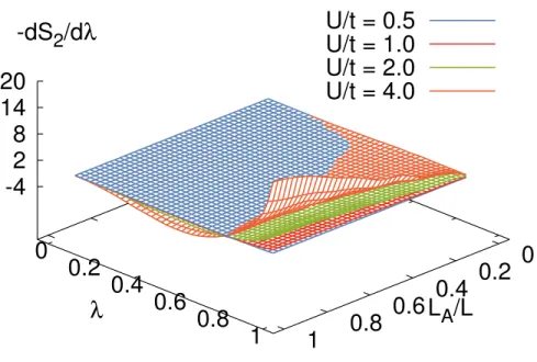
1.1 HMC results for the source (integrand) with U/t= 0.5,1.0,2.0, and 4.0 (from bottom to top at λ= 1) as functions of the auxiliary parameter λand of the region sizeLA, for a system of size

Nx= 10 sites. . . 10

1.2 Our results for the ten-site Hubbard model with couplings ofU/t= 0.5, 1.0, 2.0, and 4.0 (unbroken lines from top to bottom). Results for the noninteractingU/t= 0 case are shown using a dashed line. Hybrid Monte Carlo results, with numerical uncertainties for 7,500 decorrelated samples, are indicated by the center of their associated statistical error bars. Exact-diagonalization results from Ref. [1] are shown with lines, with the exception of theU/t= 4.0 case, where the lines join the central values of our results and are provided to guide the eye. . . 11

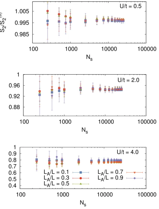
1.3 Second R´enyi entropy (in units of the noninteracting value) as a function of the number of samples Nsfor coupling strengthsU/t= 0.5, 2.0, and 4.0 shown from top to bottom. Within the first few

thousand samples, we observe that the results have stabilized comfortably to within 1-2%. . . 15

1.4 Relative statistical uncertainty of the second R´enyi entropy (propagated from the standard devi-ation in the uncertainties on its λderivative) as a function of the number of decorrelated HMC samplesNsfor coupling strengthsU/t= 0.5, 2.0, and 4.0 shown from top to bottom. The symbols

and colors correspond to those utilized above in Fig. 1.3. . . 16

1.5 Hybrid Monte Carlo results (shown with solid lines) for a ten-site, half-filled Hubbard model with U/t= 0.5, 2.0, and 4.0 and with numerical uncertainties for 7,500 decorrelated samples (for each value of λ) compared with results from the na¨ıve free-fermion decomposition method (crosses paired with dashed error bars) with 75,000 decorrelated samples. . . 17

1.6 The distribution of the natural observableQ[_{σ_}] of the na¨ıve free-fermion decomposition method [implemented via Eq. (2.7)] for coupling U/t = 2.0 and sub-system size LA/L = 0.8. We

em-phasize that the quantity Q[_{σ_}] is a non-negative one. The extended tail (main plot; note logarithmic scale in vertical axis) extends well beyond the range we have shown, and we find that it is approximately a log-normal distribution, i.e. the quantity lnQ[_{σ_}] is distributed roughly as a gaussian (inset). . . 18

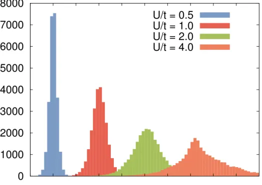
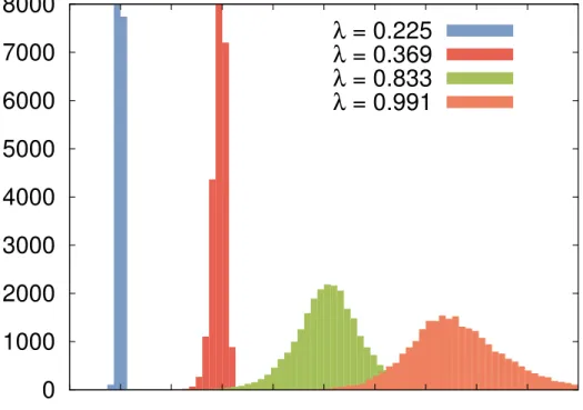
1.7 A histogram showing the distribution of our results for the derivative dS2/dλ for system size LA/L= 0.8, auxiliary parameter λ'0.83, and Hubbard couplings U/t= 0.5,1.0,2.0,4.0. The

results for different couplings have been offset relative to their true center for display purposes, but the scale is the same for each of them. This figure illustrates that, even though our method addresses the original signal-to-noise issue, strong couplings remain more challenging that weak couplings for reasons common to calculations of this type. . . 19 1.8 Histogram showing the statistical distribution of our results for the derivativedS2/dλfor system

size LA/L = 0.8, auxiliary parameter λ ' 0.225, 0.369, 0.833, 0.991, and coupling strength

2.1 Statistical distribution of the observableQ[{σ}] of the na¨ıve free-fermion decomposition method, i.e. using Eq. (2.7), for a ten-site, one-dimensional Hubbard model described by Eq. (2.33), at an attractive coupling ofU/t= 2.0 and for a subsystem of sizeLA/L= 0.8. In our case,Q[{σ}]

is a strictly non-negative quantity. The extended tail in the main plot (note logarithmic scale in vertical axis) is approximately a log-normal distribution [i.e. lnQ[_{σ_}] is roughly a normal distribution (see inset)]. . . 29 2.2 Stochastic results for_hlnQ[_{σ_}]_iλ withn= 2 for coupling strengths ofU/t= 0.5,1.0,and 2.0 as

functions of the auxiliary parameter λand the region size LA/Lfor a ten-site, one-dimensional

Hubbard model. . . 31 2.3 Results for the ten-site, one-dimensional Hubbard model for coupling strengths ofU/t= 0.5,1.0,2.0,

and 4.0 for 7,500 MC samples with associated numerical uncertainties shown. Results forU/t= 0 are depicted as a dashed line (black). For each but the largest coupling, results obtained via ex-act diagonalization from Ref. [1] are indicated by solid lines, whereas for the largest coupling, we provide a line joining the central values of our result to emphasize that its shape is consistent with results for the former and to guide the eye. . . 36 2.4 The second R´enyi entanglement entropy S2 in units of the result for a free system plotted as a

function of the number of samples Ns for coupling strengthsU/t= 0.5,1.0,2.0,and 4.0

demon-strating convergence to within a few percent within the first ten thousand samples. . . 37 2.5 R´enyi entropies Sn for n= 2,3,4 (top to bottom) of the 1D attractive Hubbard model at half

filling, as a function of the subsystem sizeLA/L. In each plot, results are shown for several values

of the attractive couplingU/t. . . 38 2.6 Stochastic results for hlnQ[{σ}]iλ with n = 2,4,6, and 8 (top to bottom) for a coupling of

U/t= 2.0 as functions of the auxiliary parameterλand the region sizeLA/L. . . 39

2.7 R´enyi entanglement entropiesSn for ordersn= 2,4,6,and 8 (top to bottom with error bars and

colors matching those in Fig. 2.6) of the 1D attractive Hubbard model at half filling, as a function of the subsystem sizeLA/L. The solid black line shows extrapolation ton= 1. The dashed black

line shows extrapolation ton_{→ ∞}. Again, results are shown for a coupling strength ofU/t= 2.0. 40 2.8 Interpolation of the R´enyi entropiesSn forn= 2,3,4, . . . ,10 for a coupling ofU/t= 2.0 given as

functions of the R´enyi ordern as well as the region sizeL_A/L. An extrapolation ton= 1 (the von Neumann entropy) as well as to n_{→ ∞}are shown in solid and dashed lines respectively. . . 41 3.1 The (bipartite) entanglement entropies computed in this work correspond to partitioning the

system into a subsystem A(in coordinate space, but it can also be defined in momentum space) and its complement in the total space ¯A. In practice, the calculations are carried out on systems that live in a periodic cubic lattice of sideL, and the subsystems are defined by cubic subregions of side LA ≤L. The reduced density matrix ˆρA of the open systemA contains the information

about entanglement betweenAand ¯A, and is obtained by tracing the full density matrix over the states supported by ¯A, which form the Hilbert space H_A¯. . . 44 3.2 Second R´enyi entropy S2 of N non-interacting fermions in d= 1,2, and 3 dimensions (top to

bottom) as a function ofx=kFLA, whereAis a segment, square, and cubic region, respectively,

3.3 Depicted here is a schematic representation of the lattice that we used in our entanglement calculations. Each horizontal lattice slice represents the three-dimensional spatial lattice where the system lives, and the vertical stacking of the planes is meant to represent the imaginary time direction. Although the original Hamiltonian is time-independent, the auxiliary fieldσthat represents the interaction is supported by a larger spacetime lattice and induces a time dependence that disappears upon averaging over this field. . . 72

3.4 The λ dependence of _hlnQ[σ]_iλ for a subsystem of size LA = 5/12L, for systems of N =

34,68,104,136,172 fermions tuned to unitarity in a box of sizeL=Nx`(where Nx= 12 points

and ` = 1), and for R´enyi order n = 2. Similar plots are obtained by varying, instead of the particle number, the region size and the R´enyi order. These are shown in Appendix .2. . . 73

3.5 Bottom panel: Low-lying entanglement spectrum of the two-body problem as a function of the dimensionless coupling (kFa)−1 in the BCS-BEC crossover regime, for a cubic subregion A of

linear size LA/L = 0.5. Top panels (a - e): Low-lying (and part of the excited) entanglement

spectrum for selected couplings (a - e) at the top of the bottom panel. . . 74

3.6 The Schmidt gap ∆ between the two largest eigenvalues of the reduced density matrix, i.e. the two smallest entanglement eigenvalues, atLA/L= 0.1,0.2, ...,0.5 (top to bottom), for the two-body

system as a function of the coupling (kFa)−1 . . . 75

3.7 The entanglement spectrum of the two-body problem in the BCS-BEC crossover regime as a function of the bare lattice coupling at a few lattice sizes: solid, dashed, dotted, dash-dotted, for Nx = 4,6,8,10, respectively. The subsystem size was fixed to LA/L = 0.5. The coupling

corresponding to the unitary point is marked with a vertical dashed line. Note how different volumes cross precisely at unitarity, which reflects the property of scale invariance characteristic of this particular system. . . 76

3.8 Top: A histogram of the higher entanglement spectrum of the two-body problem showing the number of counts (cts.) as a function of the physical coupling (kFa)−1 and the entanglement

eigenvalueλk, for region sizeLA/L= 1/2. The dashed line highlights the dependence of the mean

(see also the middle plot). Middle and bottom: The mean and standard deviation, respectively, of the high entanglement spectrum distribution, as functions of the dimensionless interaction strength (kFa)−1 (main) and kFa (inset). In each plot the different curves show results for

various region sizes LA/L. Note that the weak coupling limit corresponds tokFa→0−. . . 77

3.9 Top: The second R´enyi entanglement entropy S2 of the two-body problem as a function of x = kFLA and for several values of the coupling (kFa)−1. Inset: The entropy S2 scaled by

x2_{lnx. Bottom: The relative contribution of the high entanglement spectrum to the second} R´enyi entanglement entropyS2, as a function of x=kFLA. . . 78

3.10 The second R´enyi entropy of the resonant Fermi gas given in units ofx2_{lnx(main) andx}2_(inset), where we define the parameter x =kFLA. We note the use of a linear scale in the main plot

3.11 R´enyi entropies of order n = 2,3,4,5 (data points with error bands in red, yellow, green, and blue, respectively) of the unitary Fermi gas in units of x2_{lnx(main plot) andx}2 _{(inset), where} x = kFLA. Note the logarithmic scale in the x axis. The red dashed line shows the

non-interacting result for n= 2, obtained using the overlap matrix method. The black dotted lines plotted over the n= 2 data correspond to a fit the functional formf(x) = a+b/ln(x) (central line, with uncertainties marked by upper and lower dotted lines). The crosses on the right, and the corresponding horizontal dotted lines, indicate the expected asymptotic value c(n) (from top to bottom, forn= 2,3,4,5) for a non-interacting gas (see Refs. [2, 3, 4, 5, 6]), which we reproduce in Eq. (3.99); numerically, they are c(2) = 0.11937..., c(3) = 0.10610..., c(4) = 0.09947..., and c(5) = 0.09549.... . . 80 3.12 R´enyi entanglement entropy Sn as a function of x= kFLA for n = 2,3,4,5 (top to bottom).

Monte Carlo results are shown as data points with error bars. The solid lines show the result of computingSn using only the lowest entanglement eigenvalueλ1, i.e. the approximationSn=

n

n−1λ1. Uncertainties appear as shaded regions around the central value. . . 81 13 Top: λdependence of hlnQ[σ]iλ for several R´enyi orders n= 2,3,4,5, for subsystem sizeLA=

5/12L, for N = 172 fermions at unitarity in a box of size L=Nx` (where Nx= 12 points and

`= 1). Bottom: λdependence ofhlnQ[σ]iλ for several subsystem sizesLA, forN = 136 fermions

LIST OF ABBREVIATIONS AND SYMBOLS

A Sub-region. ¯

A Complement of sub-region.

β Temperature or imaginary time.

d Number of spatial dimensions.

GA Reduced one-body density matrix.

ˆ

H Hamiltonian operator.

HMC Hybrid Monte Carlo.

HS Hubbard-Stratonovich.

MC Monte Carlo.

n R´enyi order.

Nx Linear spatial lattice size.

QCD Quantum Chromodynamics. ˆ

ρ Density matrix.

ˆ

ρA Reduced density matrix.

Sn OrdernR´enyi entanglement entropy.

CHAPTER 1: Computing the Second R´enyi Entropy in a System of Interacting Fermions

Section 1.1: Introduction

Quantum-information and topological aspects of condensed matter physics, broadly defined in order to include all few- and many-body quantum systems, continue to gain attention from a variety of perspectives, with the notion of entanglement playing a key role [7, 8, 9]. Topological quantum phase transitions have been shown to bear a direct connection to the so-called entanglement entropy in both its von Neumann and R´enyi forms, through the entanglement spectrum, and by other information-related quantities [10, 11, 12]. Thus, the computation of R´enyi entanglement entropiesSn is currently of great importance to many fields

(see e.g. [13, 14, 15, 16, 17, 18, 19, 20]), and physicists must meet the challenge of doing so in interacting systems, particularly in strongly coupled and universal regimes.

To meet this challenge, an array of Monte Carlo (MC) methods have recently been developed to compute Sn (see e.g. [21, 22, 23, 24, 25, 26, 27, 1, 28, 29, 30, 31]). As explained below, one of the essential steps

shared accross many of the underlying formalisms is the replica trick [14], a paradigm which yields most often an expression for the entropies Sn that naturally appears as a ratio of two partition-function-like objects.

Generally, partition functions themselves are challenging objects to compute from a numerical standpoint: they typically involve terms that vary on vastly dissimilar numerical scales, a problem that only gets worse with increasing system size. In the context of stochastic calculations ofSn, it is now understood that this

complication manifests itself as a signal-to-noise problem. The na¨ıve estimation of these partition functions, followed necessarily by the calculation of their ratio, leads to unmanageable statistical uncertainties that grow exponentially with the volume of the (sub-)system considered (see e.g. [1, 28, 29] for an explanation). In this chapter, we present a lattice MC approach for the calculation of the integer-order R´enyi entropies Sn. We use a specific case of one-dimensional spin-1/2 fermions governed by a Hubbard-type Hamiltonian

dynamical fermions and has been used in a variety of graphene studies [39, 40, 41, 42].

Section 1.2: Formalism

We place the system on ad-dimensional spatial lattice of extentNx. Since we are utilizing a finite lattice,

the single-particle Hilbert space is of finite extent as well, namely Nd

x. We then follow the formalism of

Ref. [1] in order to facilitate comparison.

Then-th order R´enyi entanglement entropySnof a sub-systemAof a given quantum mechanical system

is defined as

Sn =

1

1−nln tr(ˆρ

n

A), (1.1)

where ˆρA is the reduced density matrix of sub-systemA(that is, after the degrees of freedom of the rest of

the system are traced out). Specifically, for a system with density matrix ˆρ, the reduced density matrix is defined via a partial trace over the Hilbert space corresponding to the complement ¯Aof our sub-system as

ˆ

ρA= trA¯ρ.ˆ (1.2)

Further details regarding the brute-force evaluation of this partial trace will be provided in later chapters when the few-body problem is examined in detail. We table these discussions for now.

In Ref. [1], Grover obtained an auxiliary-field path-integral form for ˆρA. Using this form, he showed

that Sn can be computed using MC methods for a range of systems. We summarize those derivations

below. In auxiliary-field Monte Carlo methods one introduces a Hubbard-Stratonovich (auxiliary) field σ that decouples the fermion species so that the usual density matrix ˆρcan be written as a path integral:

ˆ ρ=e

−βHˆ

Z =

Z

DσP[σ] ˆρ[σ], (1.3)

with

ˆ

ρA[σ] =CA[σ] exp

 −

X

i,j

ˆ c†i[ln(G

−1

A [σ]−1)]ijcˆj



, (1.5)

and where the functionalCA[σ] is defined

CA[σ] = det(1−GA[σ]). (1.6)

Above, we have used the restricted Green’s function [GA[σ]]ij, which corresponds to a free single-particle

Green’s function G(i, j) in the background fieldσ but such that the argumentsi, j only take values in the region A (see Ref. [1] and also Ref. [43, 44, 45], where expressions for the reduced density matrix of free systems, based on reduced Green’s functions, were obtained first).

Using the above choice of ˆρA[σ], Grover showed that the expectation ofcjc†i in the auxiliary free system

correctly reproduces the restricted single-particle Green’s functions, as it is required to do. Therefore, by linearity, expectation values of observables supported only in the region A are reproduced as well. This validates the expression on the right-hand side of Eq. (2.4).

Using this expression, taking powers of ˆρAnecessarily results in the appearance of a number of HS fields,

which we collectively denote below as _{σ_}. A manifestation of the replica trick [14], this approach allows the trace of the n-th power of ˆρA in Eq. (2.1) to be recast as a field integral over a product of fermion

determinants that depend on the collection of fields_{σ_}. Indeed, for a system of 2N-component fermions, using an auxiliary-field transformation that decouples them, we obtain

exp (1₋n)Sn

=

Z

D{σ_}P[_{σ_}]Q[_{σ_}], (1.7)

where the field integration measure, given by

D{σ} =

n

Y

k=1 Dσ_k

Z , (1.8)

is over then”replicas”σ_k of the Hubbard-Stratonovich auxiliary field. We have included the normalization

Z=

Z

Dσ 2N

Y

m=1

detUm[σ] (1.9)

factorizes completely across replicas, and it is therefore blind to correlations associated with quantum entan-glement. This factorization is the main reason why using P[{σ}] as a MC probability leads to (seemingly) insurmountable signal-to-noise problems, as shown in Ref. [1]; it is also why we call it na¨ıve (although that is by no means a judgement of Ref. [1]). In Eq. (2.10),Um[σ] is a matrix which encodes the dynamics of the

m-th component in the system, namely the kinetic energy and the form of the interaction after an auxiliary-field decomposition; it further encodes the form of the trial ket_|Ψ_iin ground-state projective formulations (see e.g. Ref. [32, 33, 34]), as we employ in this work. We will take the ket_|Ψ_ito be a Slater determinant. In finite-temperature approaches, the matrixUm[σ] is obtained by evolving a complete set of single-particle

states in imaginary time.

The factor that introduces the critical contributions to entanglement measures is

Q[_{σ_}] = 2N

Y

m=1

detMm[{σ}], (1.11)

where we abbreviate

Mm[{σ}]≡ n

Y

k=1

1₋GA,m[σk]

"

1 +

n

Y

k=1

GA,m[σk]

1₋G_A,m[σ_k]

#

. (1.12)

In the above equation, we have writtenGA,m[σk], which is a restricted Green’s function, as previously defined,

but where we now indicate the fermion componentmand replica field indexk.

The product Q[_{σ_}] was identified as playing the role of an observable in Ref. [1], which is a natural interpretation in light of Eq. (2.7), but which we will interpret differently below. Note that, for n= 2, thankfully, no matrix inversion is required in the calculation of Q[{σ}]; for higher n, however, there is no obvious way to avoid the inversion of 1−GA,m[σk]. We comment on this in subsequent chapters. Otherwise,

it seems this calculation would require some kind of numerical regularization technique (see Ref. [30, 31]) to avoid singularities inGA,m[σk], whose eigenvalues can be close to zero and unity.

In zero-temperature paradigms, the extent of Um[σ] is given by the number of particles of the m-th

species present in the system. In finite-temperature approaches, the size is that of the whole single-particle Hilbert space (i.e. the size of the lattice, as mentioned earlier). The size of GA,m[σk], on the other hand,

Section 1.3: Our proposed method

By analogy to the right side of Eq. (2.7), we define an auxiliary parameter 0 _≤λ_≤1 and introduce a function Γ(λ;g) as

Γ(λ;g)≡

Z

D{σ}P[{σ}]Q[{σ};λ], (1.13)

where we have augmented the dependence ofQ[{σ}] on the coupling g by replacing

g_→λ2_{g, (1.14)}

which defines Q[_{σ_};λ]. From this definition, it follows immediately that Γ(λ;g) satisfies two pivotal con-straints, each of which with different nontrivial physical significance: Forλ= 0, we see

1

1₋nln Γ(0;g) =S (0)

n , (1.15)

where Sn(0) is the entropy of a noninteracting system, that is, one where g → 0. To wit, at λ = 0 the

functional Q[{σ};λ] does not depend on the auxiliary fields {σ} and factors completely from the integral. Ergo, independent of the numerical value ofg, the function Γ(0;g) corresponds to the R´enyi entropy of a free system, which can be computed trivially within the present formalism, although in the prototype calculations that follow, we make use of Grover’s original formalism for simplicity. Indeed, in the free case the lack of fluctuation in the auxiliary field implies that there is no path integral when interactions are turned off, such that the noninteracting result can be computed with a single Monte Carlo sample using the formalism by Grover mentioned above. It is worth mention that the R´enyi entropy of a noninteracting system has received substantial attention in the recent few years, with specific techniques developed for their study and specific, and interesting, results arising therefrom. A lot is known about these quantities for a variety of systems, in particular in connection with area laws, modified area laws, and their violation [2, 3, 46, 4, 6].

For λ = 1, on the other hand, Γ(λ;g) corresponds to the R´enyi entanglement entropy of the fully interacting system:

1

1₋nln Γ(1;g) =Sn. (1.16)

where

˜

P[{σ};λ] = 1

Γ(λ;g)P[{σ}]Q[{σ};λ], (1.18) and

˜

Q[_{σ_};λ] = 2N

X

m=1 tr

M_m,λ−1[_{σ_}]∂Mm,λ[{σ}] ∂λ

. (1.19)

It is important that any dependence on the auxiliary parameter λappears only in the matrixMn. It is in

this way that we include the entanglement correlations in the MC sampling algorithm, which is to be done using ˜P[_{σ_};λ] as the probability measure. When considering an even number of flavors 2N, and when the interactions are not repulsive, det2NU[σ] and Q[_{σ_}, λ] are real and positive semidefinite for any real σ. This nonnegativity means that there is no sign problem, and ˜P[{σ};λ] above is useful as a normalized, well-defined probability distribution.

More specifically, the method presented in this chapter to computeSn is to take the freeλ= 0 point as

a reference and calculateSn by integration using

Sn=Sn(0)+

1 1₋n

Z 1

0

dλhQ[˜ {σ};λ]i, (1.20)

where

hX_i=

Z

D{σ_}P˜[_{σ_};λ]X[_{σ_}]. (1.21)

Another way, we obtained an integral form of the interacting R´enyi entanglement entropy that can be calculated using any of a great variety of MC methods, in particular the hybrid Monte Carlo algorithm (HMC) [35, 36]. The latter combines molecular dynamics (MD) of the auxiliary fields (defining a fictitious auxiliary conjugate momentum independent of the auxiliary fields) with the Metropolis-type accept-reject step. This combination enables simultaneous global updates of alln of the auxiliary fields{σ}. As is well known in the lattice QCD community, HMC is an exceptionally efficient sampling strategy, particularly when gauge fields are required (see e.g. [35, 36, 32, 33, 34]). The integration of the MD equations of motion requires the calculation of the MD force, which is given by the functional derivative of the augmented measure

˜

P[_{σ_};λ] with respect to the fields_{σ_}, and can be calculated directly from Eq. (3.88).

is that the expectation that appears above is taken with respect to the augmented probability measure ˜

P[{σ};λ] , which includes the correlations that account for quantum entanglement. In contrast to the na¨ıve MC probability P[{σ}], which corresponds to statistically independent replicas of the auxiliary field, this measure does not display the factorization responsible for the signal-to-noise problem afflicting previous work mentioned above.

In practice, using Eq. (3.89) requires MC calculations to evaluatehQ[˜{σ};λ]istochastically as a function of the parameter λ, followed by numerical integration over this parameter. We find that _hQ[˜ _{σ_};λ]_i is a surprisingly smooth function ofλthat vanishes gradually atλ= 0 and displays most of its features close to λ= 1 (further details below). We therefore carry out the numerical integration using the Gauss-Legendre quadrature method [47] in an effort to sample it efficiently. It should also be pointed out that the stochastic evaluation of_hQ[˜_{σ_};λ]_i, for fixed subregionA, can be expected to feature roughly symmetric fluctuations about its mean value. Therefore, after integration over the parameterλ, the statistical effects on the entropy are reduced (as we show empirically in the Results section of this chapter).

A few comments are necessary at this point regarding the auxiliary parameter. First, we could have performed the replacementg_→λ2_{geverywhere, i.e. not only inQbut also inP(including its normalization} Z). This global replacement would have led to three terms in the derivative of P Q with respect to λ, two of which would come fromP (recall P is normalized) and feature different signs and a rather indirect connection to Sn (recall P factorizes across replicas). Our approach avoids this superfluous difficulty by

focusing solely on the entanglement portion of the integrand (i.e. Q). Additionally, we could have used a power λx _{of the auxiliary parameter rather than its square λ}2_{, where xdoes not have to be an integer} (although it would be rather inconvenient to make it less than 1). This is indeed a possibility, and it allows for further optimization than pursued here. In what remains of this chapter, we setx= 2, as above. Finally, the calculations required for different values ofλare completely independent from one another with likely unrelated probability measures governing their evaluation. These calculations can therefore be performed wholly in parallel with essentially perfect scaling (up to the computationally negligible final data gathering and quadrature).

the calculation begins from the replica trick originally introduced by Calabrese and Cardy [14], i.e.

exp((1−n)Sn) =

ZA,n

Zn , (1.22)

where_ZA,nis the partition function ofnreplicas of the system ”glued” together across the quantum numbers

A. Usually,_ZA,nandZncan be grossly different from each other in scale, especially ifSnis large (as is usually

the case for large sub-system sizes). As a result, calculating the partition functions given above separately (and stochastically) and attempting afterward to evaluate the ratio of the two is very likely to yield a large statistical uncertainty resulting in a significant signal-to-noise problem. Hope of circumventing this problem is can be derived from the use of the ratio (or increment) trick, whereby one introduces auxiliary ratios of the partition function corresponding to systems whose configuration spaces are only marginally dissimilar. In other words, one uses

exp((1₋n)Sn) =

ZA,n

Zn =

ZA,n

ZA−1,n

ZA−1,n

ZA−2,n

· · ·Z2,n Z1,n

Z1,n

Zn , (1.23)

where the intermediate ratios _ZA−i,n/ZA−i−1,n are chosen to correspond to subsystems of similar size and

shape (e.g. such that their linear dimension differs by one lattice spacing). In this way, each of the auxiliary ratios can be expected to not differ significantly from unity, and with enough intermediate ratios, calculations can be carried out in a stable fashion at the price of calculating a potentially large number of ratios.

In the method we detail here, the auxiliary parameterλis analogous to the varying region sizeAof the ratio trick. Using Eq. (3.89), we may write

exp(1₋n)(Sn−S

(0)

n )

= 1

Y

λ=0

exp∆λ_hQ[˜_{σ_};λ]_i, (1.24)

where any discretization ∆λ of the exponent inside the product yields an acceptable (similar) telescoping sequence of ratios as in Eq. (1.23). So long as_hQ[˜ _{σ_};λ]_iis regular inλ, which we find to be the case in all work performed, our auxiliary factors can be made to be arbitrarily close to unity at the cost of (at most) linear scaling in computation time.

operator we simulate is

ˆ

H =−t X

s,hiji

ˆ

c†i,scˆj,s+ ˆc

†

j,sˆci,s

+UX

i

ˆ

ni↑nˆi↓, (1.25)

where in the above the first sum includes our two distinct fermion speciess=_↑,_↓ and all pairs of nearest-neighbor sites. We implemented a symmetric (second order) Trotter-Suzuki factorization of the original canonical Boltzmann weight, with an imaginary-time discretization parameter τ = 0.05 (in lattice units). The full extent of the imaginary-time axis was at its largest β = 5 (that is, we had 100 imaginary-time lattice sites). The factor in the Trotter-Suzuki decomposition that contains the interaction was addressed, as anticipated in a previous discussion, by introducing a replica HS variableσfor each power of the reduced density matrix ˆρ_A. This insertion was accomplished by an auxiliary-field transformation. We selected a version of this transformation based around a continuous field with a convenient, compact range (see Ref. [32, 33, 34]).

Figure 1.1 shows the MC average hQ[˜ {σ};λ]i as a function of not only the auxiliary parameter λ but also of the subregion size LA for four values of the Hubbard coupling U/t. We emphasize that surfaces

corresponding to weak couplings demonstrate significantly less fluctuation along both axes than do their strongly interacting analogues. This uniformity suggests that for weakly coupled systems, even at largeLA,

a coarseλdiscretization may yield accurate estimates of Sn. Conversely, strongly coupled systems are, not

unexpectedly, more computationally demanding.

U/t = 0.5

U/t = 1.0

U/t = 2.0

U/t = 4.0

0

0.2

0.4

0.6

0.8

1

L

_A

/L

0

0.2

0.4

0.6

0.8

1

λ

-4

2

8

14

20

-dS

₂

/d

λ

Figure 1.1: HMC results for the source (integrand) withU/t= 0.5,1.0,2.0, and 4.0 (from bottom to top at λ= 1) as functions of the auxiliary parameterλand of the region sizeLA, for a system of sizeNx= 10 sites.

Our experience with this method, and this system in particular, indicates that the features we have observed in studying the source_hQ[˜ _{σ_};λ]_iare quite generic: they fluctuate in amplitude with the coupling, but their qualitative features are largely insensitive to the overall system size, and they generally behave in a surprisingly benign way as a function of λ and the sub-system size, so long as the sampling routine is sufficiently robust. Hence, the auxiliary parameter integration does not contribute to the scaling of the computation time versus system size beyond a manageable prefactor. We present our results upon integrating overλas detailed above in the section that follows.

1.5.1: Comparison with exact diagonalization results and a look at statistical effects

In Fig. 1.2, we depict results for a system of size L=Nx`, withNx = 10 sites and a lattice spacing of

`= 1 as in conventional Hubbard-model studies. These calculations include couplings U/t= 0.5, 1, 2, and 4, and subsystems of sizesLA = 1−10. We compare our results to the results given in Ref. [1], and the

1

1.2

1.4

1.6

1.8

2

2.2

0

0.2

0.4

0.6

0.8

1

S

2

(L

A

)

L

_A

/L

U/t = 0.5

U/t = 1.0

U/t = 2.0

U/t = 4.0

Figure 1.2: Our results for the ten-site Hubbard model with couplings of U/t = 0.5, 1.0, 2.0, and 4.0 (unbroken lines from top to bottom). Results for the noninteractingU/t= 0 case are shown using a dashed line. Hybrid Monte Carlo results, with numerical uncertainties for 7,500 decorrelated samples, are indicated by the center of their associated statistical error bars. Exact-diagonalization results from Ref. [1] are shown with lines, with the exception of theU/t= 4.0 case, where the lines join the central values of our results and are provided to guide the eye.

given exceptional results. These figures show that, by including the entanglement-sensitive factor into the probability measure itself, our approach circumvents the devastating signal-to-noise problem mentioned in the introduction, making the sampling procedure enormously more efficient and the calculation manageable. Below we elaborate more explicitly on statistical effects and on this noise problem, and we include concrete numerical examples of how it arises in calculations.

1.5.2: Comparison with na¨ıve free-fermion decomposition method

Figure 1.5 depicts again the results for our half-filled, ten-site Hubbard model using 7,500 decorrelated samples for each value of the parameterλ, and this time, it offers a comparison with the na¨ıve free-fermion decomposition method using a comparable 75,000 samples. Such an increased number of samples for the na¨ıve method was selected to offer a more balanced comparison with our method, as the latter technique requires a MC calculation for each value ofλ, but those calculations are independent. We used 20λpoints but, as explained in more detail below, roughly half of theλpoints require only a small number of samples to achieve reasonable accuracy and precision.

Often, the statistical uncertainties associated with the na¨ıve calculation do not contain the expected values for the entropy. This disagreement is symptomatic of an ”overlap” problem, a situation where the probability measure used bears little to no correlation with the observable of interest, as already mentioned once above (see also Ref. [48]). This situation is the same as the signal-to-noise problem referred to in preceding discussions.

To illustrate this issue more precisely, we show in Fig. 2.1 a histogram ofQ[{σ}] [see Eq. (2.7)] for coupling U/t = 2.0 and system size LA/L = 0.8. Even after using a logarithmic vertical scale, the distribution of

Q[_{σ_}] displays an extended tail that survives across numerous orders of magnitude. We find that the distribution is approximately of the log-normal type (that is, its logarithm is approximately distributed as a gaussian, as shown in the inset of Fig. 2.1); this situation presents a great challenge when the average of Q[_{σ_}] must be determined with good precision by means of implementing the free-fermion decomposition of Ref. [1] in its purest form. Additionally, we further expect these features to worsen quickly in larger systems, especially in higher dimensions and at stronger couplings, as the matrices involved become more and more ill-conditioned and the scaling of the entropy, as seen in free systems, shifts toward more and more potent divergences of the power-law variety.

We emphasize that it is the logarithm of the average ofQ[_{σ_}] that determines the quantities of interest, a quantity which could then be obtained by means of the cumulant expansion; however, it is a priori entirely unknown whether such an expansion would converge if it can even be carried out, as there is no knowledge of to what extent the qualities of this distribution deviate from gaussianity.

problems are characterized by the heavy tail of a lognormal distribution (see also, Ref. [49]), and in some cases this behavior has been exploited to provide physical insights.

1.5.3: Statistical behavior as a function of coupling, region size, and auxiliary parameter

In Fig. 1.7 we give the statistical distribution of our results for the λ derivative for several values of the coupling. These distributions are in most cases approximately gaussian (that is, their tails decay faster than linearly in a log scale), except for the strongest coupling we studied U/t = 4.0 where, not entirely unexpectedly, the distribution becomes more asymmetric and develops extended tails relative to its weaker-coupling analogues.

In Fig. 1.8 we show the distribution of our results for the λ derivative at fixed sub-system size and coupling strength, but we varyλ. As stated previously, the parameterization we chose requires considerably fewer decorrelated MC samples at lowerλthan at higherλ, as the width of the distributions is much smaller for the former than it is for the latter.

Lastly, in Fig. 1.9 we illustrate the same distribution as above, but as a function of sub-system size. As anticipated, larger subregions are more challenging, but the overall shape of the distributions is very well controlled: it remains close to gaussian in that its tails decay faster than linearly in a log scale, a significant improvement over the distributions shown earlier.

Section 1.6: Summary and Conclusions

In this chapter, we have described an alternative MC approach to the calculation of the R´enyi entangle-ment entropy of many-fermion systems. A central component of this method is to compute the derivative of the entanglement entropy with respect to an auxiliary parameter and integrate afterwards to compute the difference between the interacting and non-interacting entropies. We have demonstrated that such a derivative can be calculated through a MC method without the previously observed signal-to-noise issues, as the resulting expression yields a probability measure that does not factor across replicas and accounts for entanglement-sensitive correlations in the MC sampling procedure in an efficient, natural way. The required numerical integration can be carried out by any of numerous well-known methods, and in the present case, we computed the required quadratures by means of the Gauss-Legendre rule.

0.985

0.995

1.005

100

1000

10000

100000

S

/S

2

(0)

N

U/t = 0.5

0.88

0.92

0.96

1

100

1000

10000

100000

N

U/t = 2.0

0.4

0.5

0.6

0.7

0.8

0.9

1

100

1000

10000

100000

N

U/t = 4.0

L

/L = 0.1

L

/L = 0.3

L

/L = 0.5

L

/L = 0.7

L

/L = 0.9

Figure 1.3: Second R´enyi entropy (in units of the noninteracting value) as a function of the number of samplesNs for coupling strengths U/t= 0.5, 2.0, and 4.0 shown from top to bottom. Within the first few

0.1

1

100

1000

10000

100000

∆

S

N

1/2

/S

2

(0)

N

U/t = 0.5

0.1

1

10

100

1000

10000

100000

N

U/t = 2.0

1

10

100

1000

10000

100000

N

U/t = 4.0

Figure 1.4: Relative statistical uncertainty of the second R´enyi entropy (propagated from the standard deviation in the uncertainties on itsλderivative) as a function of the number of decorrelated HMC samples Ns for coupling strengths U/t = 0.5, 2.0, and 4.0 shown from top to bottom. The symbols and colors

1.2

1.4

1.6

1.8

0

0.2

0.4

0.6

0.8

1

S

(L

)

L

/L

U/t = 0.5

1.2

1.4

1.6

1.8

0

0.2

0.4

0.6

0.8

1

L

/L

U/t = 2.0

0.7

0.9

1.1

1.3

1.5

0

0.2

0.4

0.6

0.8

1

L

/L

U/t = 4.0

Q

1

10

100

1000

10000

5

10 15 20 25 30 35 40 45 50 55

ln Q

0

20000

40000

60000

80000

-12

-6

0

6

Figure 1.6: The distribution of the natural observableQ[_{σ_}] of the na¨ıve free-fermion decomposition method [implemented via Eq. (2.7)] for couplingU/t= 2.0 and sub-system sizeLA/L= 0.8. We emphasize that the

U/t = 0.5

U/t = 1.0

U/t = 2.0

U/t = 4.0

0

1000

2000

3000

4000

5000

6000

7000

8000

Figure 1.7: A histogram showing the distribution of our results for the derivative dS2/dλ for system size LA/L= 0.8, auxiliary parameterλ'0.83, and Hubbard couplingsU/t= 0.5,1.0,2.0,4.0. The results for

λ

= 0.225

λ

= 0.369

λ

= 0.833

λ

= 0.991

0

1000

2000

3000

4000

5000

6000

7000

8000

Figure 1.8: Histogram showing the statistical distribution of our results for the derivativedS2/dλfor system size LA/L= 0.8, auxiliary parameterλ'0.225, 0.369, 0.833, 0.991, and coupling strengthU/t= 2.0. Our

L

_A

/L = 0.1

L

_A

/L = 0.3

L

_A

/L = 0.5

L

_A

/L = 0.8

0

1000

2000

3000

4000

5000

6000

7000

8000

Figure 1.9: A histogram showing the distribution of our results for the derivativedS2/dλfor regions of size LA/L=0.1, 0.3, 0.5, 0.8, auxiliary parameters ofλ'0.83, and a coupling strength ofU/t= 2.0. The results

CHAPTER 2: Higher Order Entropies and a More Stable Algorithm

Section 2.1: Introduction

In the previous chapter, we detailed an algorithm to calculate the R´enyi entanglement entropies Sn of

interacting fermion models. Numerous other algorithms have been proposed during the last few years to this effect [16, 21, 22, 24, 25, 26, 28, 29, 27]. This chapter’s method, based on Grover’s free-fermion decomposition formalism given originally in our Ref. [1], alleviates the signal-to-noise problem present in that algorithm, and our second method is also compatible with the hybrid Monte Carlo (HMC) workhorse [37, 38, 35, 36] extensively utilized in the context of lattice quantum chromodynamics (QCD) and other gauge-field-based simulations. The central point of the last chapter’s method is that, by differentiating with respect to an auxiliary parameter λ, one may carry out a Monte Carlo (MC) calculation of dSn/dλ with a probability

measure that includes entanglement-sensitive correlations explicitly. [This circumvention was certainly not the case in the approach of Ref. [1], where the probability measure factored completely across the multiple auxiliary field replicas; we identified this factorization as the primary cause of this particular, and particularly devastating, signal-to-noise problem (see discussion that follows)]. After the MC calculation is complete, (numerical) integration with respect to the auxiliary parameter λ returns the desired R´enyi entanglement entropy relative to that of a noninteracting system (which is easily computed separately); that is, it returns the contribution to the R´enyi entropies coming from the presence of the interactions.

entropiesSn, and thus brings to the forefront the approximate lognormality property which was mentioned

above.

In what follows, we present our basic formalism, review our evidence for approximately lognormal dis-tributions, and explain our method. In addition to the points mentioned above, in our computations we have found the present method to be much more numerically stable than its predecessor in the sense that it functions more smoothly with more lenient MC input parameters. We explain this in detail in this chapter’s Results section.

In addition to the new, more elegant method, we demonstrate that it is possible to rewrite part of the formalism in order to bypass the calculation of inverses of the restricted density matrix (see e.g. [28, 29]) in the determination of R´enyi entropies of ordern >2, a problem highlighted in the literature and one which causes great difficulty in the computation of higher order entropies. To test our method, we computed the n= 2 R´enyi entropy of the attractive one-dimensional Hubbard model using the previous formalism as well as the new formalism and we checked that we obtained identical results. In going further than the n = 2 case, we present results for then = 2,3,4, . . . ,10 R´enyi entropies, and we see that higher R´enyi entropies display reduced statistical uncertainty in MC calculations. Finally, we attempt an extrapolation to large and small R´enyi orders.

Section 2.2: Basic formalism

As in the previous chapter, we quickly set the stage by presenting the formalism of Grover’s method originally put forward in Ref. [1]. Then-th R´enyi entropySn of a sub-systemAof a given model is given by

Sn =

1

1₋nln tr(ˆρ

n

A), (2.1)

where ˆρ_A is the reduced density matrix of the sub-system A. For a system with canonical density matrix ˆ

ρ, the reduced density matrix is defined via a partial trace over the Hilbert space corresponding to the complement ¯A of our sub-system in the full set of quantum numbers:

ˆ

ρA= trA¯ρ.ˆ (2.2)

field integral by means of a Hubbard-Stratonovich (HS) auxiliary-field transformation:

ˆ ρ=e

−βHˆ

Z =

Z

DσP[σ] ˆρ[σ], (2.3)

for a normalized probability measureP[σ] determined by the details of the underlying model’s Hamiltonian (for more detail, see below and also Ref. [32, 33, 34]). In the above expression,_Z is the partition function, and ˆρ[σ] is the density matrix of a system of noninteracting fermions in the fixed external auxiliary fieldσ. One of the central advances of Ref. [1] was to demonstrate that this decomposition determines not only the full density matrix but also the restricted one and, crucially, all associated one-body correlations. Indeed, Ref. [1] shows that

ˆ ρA=

Z

DσP[σ] ˆρA[σ], (2.4)

whereP[σ] is the same probability used in Eq. (2.3),

ˆ

ρA[σ] =CA[σ] exp

 −

X

i,j

ˆ c†i[ln(G

−1

A [σ]−1)]ijcˆj



, (2.5)

and

CA[σ] = det(1−GA[σ]). (2.6)

In the above, we denote by GA[σ] the restricted Green’s function of the free system in the external

background fieldσ(see below), and ˆc†_{, ˆc are the fermion creation and annihilation operators. The sums in} the exponent of Eq. (2.5) range over those points in the system which belong to the subsystemA.

By using the above formalism for the case of 2N-component fermions, the R´enyi entropy (c.f. Eq. 2.1) becomes

exp (1₋n)Sn

=

Z

D{σ_}P[_{σ_}]Q[_{σ_}], (2.7)

where the field integration measure, given by

representation of ˆρA shown above, and the normalization Z= Z Dσ 2N Y m=1

detUm[σ] (2.9)

was included in the measure. It is worth explicitly mentioning that, by separating out a factor of_Zn _{in the}

denominator of Eq. (2.7), an explicit form can be identified in the numerator as in the replica trick [14], which corresponds to a ”replica” partition function forncopies of the system, ”glued” together in the region Aas a result of the particular structure of the matrix product and partial trace.

The na¨ıve probability measure, namely

P[_{σ_}] =

n Y k=1 2N Y m=1

detUm[σk], (2.10)

factorizes completely across replicas, which makes it largely insensitive to entanglement-oriented correlations. This factorization is the central reason why using P[_{σ_}] as the MC probability leads to signal-to-noise problem (see Ref. [1]). In Eq. (2.10),Um[σ] encodes the dynamics of them-th fermion species, including the

kinetic energy and the form of the interaction after a Hubbard-Stratonovich transformation. This matrix also encodes the form of the trial state|Ψiin imaginary-time-projective, ground-state approaches (see e.g. Ref. [32, 33, 34]), a version of which we use here; in what follows, we have taken|Ψito be a Slater determinant of single-particle orbitals. In finite-temperature approaches,Um[σ] is obtained by evolving a complete set of

single-particle states in imaginary time.

The quantity that contains the critical input to the entanglement entropy is the determinant

Q[{σ}] = 2N

Y

m=1

detMm[{σ}], (2.11)

which we refer to below as the ”entanglement determinant,” and where the matrixMm[{σ}] is given by

Mm[{σ}]≡ n

Y

k=1

1₋GA,m[σk]

× " 1 + n Y l=1

GA,m[σl]

1₋G_A,m[σ_l]

#

. (2.12)

to match (see Ref. [1] and also Ref. [43, 44, 45], where expressions were originally derived for the reduced density matrix of noninteracting systems, based on reduced Green’s functions).

Section 2.3: Avoiding inversion of the reduced Green’s function for n >2

Addressed explicitly in Ref. [30, 31], for n= 2, no inversion of the difference 1−GA,m[σk] is actually

required in the calculation of the entanglement determinantQ[_{σ_}], as straightforward calculation immedi-ately confirms that the equations simplify in that case. However, for highernit is not at all obvious how to avoid such an inversion or if it can be avoided at all. Below, we demonstrate that this calculation can indeed be accomplished without performing this troublesome inversion. We begin by factoring the entanglement determinant such that

detMm[{σ}] = detLm[{σ}]detKm[{σ}], (2.13)

whereLm[{σ}] is a block diagonal matrix (one block per replicak):

Lm[{σ}]≡diag

1−GA,m[σk]

, (2.14)

and

Km[{σ}]≡

            

1 0 0 . . . 0 −R[σn]

R[σ1] 1 0 . . . ... 0

0 R[σ2] 1 0 0 0

..

. . .. . .. ... 1 ...

0 . . . 0 R[σn−1] 1

             , (2.15)

where the ones in the above are identity matrices and where we have defined

R[σk] =

GA,m[σk]

first r.h.s. factor in the first line of Eq. (2.12); the remaining factor relies on the identity det             

1 0 0 . . . 0 Hk

−H1 1 0 . . . ... 0

0 ₋H2 1 0 0 0

..

. . .. ... ... 1 ... 0 . . . 0 −Hk−1 1

            

= det (1 +H1H2. . . Hk), (2.17)

which is valid for arbitrary block matricesHj, is a standard result often used in many-body physics (especially

when implementing a Hubbard-Stratonovich transformation), and can be shown using so-called elementary operations on rows and columns.

Within the determinant of Eq. (2.13), we multiply Km[σ] andLm[σ]:

Tm[{σ}]≡Km[{σ}]Lm[{σ}] = 1− Gm[{σ}]B, (2.18)

where_Gm[{σ}] is a block diagonal matrix defined by

Gm[{σ}] = diagGA,m[σn]

, (2.19) and B_≡             

1 0 0 . . . ₋1 1 1 0 . . . 0 0 1 1 . . . 0 ..

. . .. ... ... ... 0 . . . 0 1 1

             (2.20)

where again the ones given in the above are identity matrices. Equation (2.18) proves our claim, as we may useTm[{σ}] in our calculations instead ofMm[{σ}], and the former contains no inverses of 1−GA,m greatly

simplifying the calculation of higher order entropies.

Summarizing, a class of approaches to calculating Sn for n > 2, based on the Hubbard-Stratonovich

[Eq. (2.13) and beyond] we have demonstrated that no inversions are actually required, asTm[{σ}] contains

no inverses and because its determinant is equivalent to the original, more computationally unstable, form. While this is a desirable feature from a numerical point of view, it should be mentioned that, from a computational-cost point of view, the price of not inverting 1₋GA,m reappears in the fact thatTm, though

sparse, scales linearly withnin size.

For the remainder of this chapter, all calculations carried out at n = 2 use theM-approach, which is based on Eq. (2.12) and the ’proposed method’ described below. We reproduced those results by switching to the T-approach, which uses Eq. (2.18) (as well as the method described below), and we then proceeded to highernwith the latter formulation.

Section 2.4: A statistical observation: lognormal distribution of the entanglement determi-nant

In the previous chapter, we offered examples of the approximate log-normal distributions obeyed by Q[_{σ_}] when sampled according to the na¨ıve measureP[_{σ_}]. One specific example is reproduced here for reference in Fig. 2.1. The fact that such statistical distributions are approximately log-normal, at least visually, strongly suggests that one may use the cumulant expansion to determineSn. Generally,

(1₋n)Sn = ln

Z

D{σ_}P[_{σ_}]Q[_{σ_}]

= ∞

X

m=1

κm[lnQ]

m! , (2.22)

whereκm[lnQ] is them-th cumulant of lnQ, and the first two nontrivial cumulants are given by

κ1[X] =hXi (2.23)

and

κ2[X] =hX 2

i − hX_i2 _(2.24)

Q

1

10

100

1000

10000

20

40

60

80

100

120

Ln Q

0

25000

50000

75000

-12

-6

0

6

Figure 2.1: Statistical distribution of the observableQ[_{σ_}] of the na¨ıve free-fermion decomposition method, i.e. using Eq. (2.7), for a ten-site, one-dimensional Hubbard model described by Eq. (2.33), at an attractive coupling ofU/t= 2.0 and for a subsystem of sizeLA/L= 0.8. In our case,Q[{σ}] is a strictly non-negative

quantity. The extended tail in the main plot (note logarithmic scale in vertical axis) is approximately a log-normal distribution [i.e. lnQ[_{σ_}] is roughly a normal distribution (see inset)].

fluctuate wildly across a huge range of scales), they are very difficult to determine stochastically (the signal-to-noise problem re-emerges in a different form), and there is currently no easy way to obtain clean analytic insight into the large-m behavior ofκm. Nevertheless, this approximate log-normality does provide a path

forward, as it indicates that we may still evaluate hlnQito good precision with MC methods. As we will demonstrate in the next sections, this evaluation is enough to determineSnif we are willing to pay the price

of a one-dimensional integration on a compact domain.

Section 2.5: Proposed method

Beginning from the right side of Eq. (2.7), we introduce an auxiliary variable 0_≤λ_≤1 and define a new function Γ(λ;g), analogous to the one defined in the previous chapter, via

Γ(λ;g)_≡

Z

D{σ_}P[_{σ_}]Qλ_[

{σ_}]. (2.25)

Atλ= 0,

ln Γ(0;g) = 0, (2.26)

while atλ= 1, Γ(λ;g) provides the full R´enyi entanglement entropy:

1

1−nln Γ(1;g) =Sn. (2.27)

From Eq. (3.84),

∂ln Γ ∂λ =

Z

D{σ_}P˜[_{σ_};λ] lnQ[_{σ_}] (2.28)

where

˜

P[_{σ_};λ] = 1

Γ(λ;g)P[{σ}]Q

λ_[

{σ_}]. (2.29)

With an even number of species 2N and with attractive interactions, the quantities P[{σ}] and Q[{σ}] are wholly real and strictly non-negative for all fields σ, such that there is no sign problem and such that

˜

P[{σ};λ] above is a well-defined and normalized probability measure.

As in the previous chapter, using this, we can computeSn by taking the initialλ= 0 point as a reference

and computing the entropy from

Sn =

1 1−n

Z 1

0

dλhlnQ[{σ}]iλ, (2.30)

where we have defined

hX_iλ=

Z

D{σ_}P[˜ _{σ_};λ]X[_{σ_}]. (2.31)

Thus, we arrive at an integral form for the fully interacting R´enyi entanglement entropy that can be computed using any MC method (see e.g. [32, 33, 34]), in particular HMC [35, 36, 37, 38].

U/t = 0.5

U/t = 1.0

U/t = 2.0

0

0.2

0.4

0.6

0.8

1

L

_A

/L

0

0.2

0.4

0.6

0.8

1

λ

-2

-1

0

1

dln

Γ

/d

λ

Figure 2.2: Stochastic results for _hlnQ[_{σ_}]_iλ with n= 2 for coupling strengths of U/t= 0.5,1.0, and 2.0 as functions of the auxiliary parameterλand the region sizeLA/Lfor a ten-site, one-dimensional Hubbard

model.

Stratonovich field, this admittedly more complicated statistical distribution does not exhibit the factorization responsible for the signal-to-noise problems present in the approach as it was originally written down.

Making use of Eq. (3.89) requires a Monte Carlo method to evaluate the expectation value_hlnQ[_{σ_}]_iλas

a function ofλ, followed by numerical integration over this superfluous parameter. As in the last chapter, we see here that_hlnQ[_{σ_}]_iλis a surprisingly smooth function ofλ, which is essentially linear in the present case.

It is therefore sufficient to perform the numerical integration using a uniform grid rather than a specialized quadrature as was done above. In the chapter that follows, we will again find surprisingly linear behavior as a function of λand will use a uniform grid in that case as well. The stochastic evaluation of the source hlnQ[{σ}]iλ, for fixed subregion A, can be expected to feature roughly symmetric fluctuations about the

point

∂ln Γ ∂λ

_λ=0 =

Z

D{σ}P[{σ}] lnQ[{σ}] (2.32)

≤ ln

Z

D{σ}P[{σ}]Q[{σ}] = (1−n)Sn,

which must be satisfied by our calculations. Our Monte Carlo results atλ= 0 do indeed satisfy this bound.

Section 2.6: Results

2.6.1: Second R´enyi entropy

As a first test of our algorithm and in efforts to make contact with previous work [1], we begin by showing results for the second R´enyi entropy S2 for the one-dimensional, half-filled Hubbard model with periodic boundary conditions, whose Hamiltonian operator is

ˆ

H =₋t X

s,hiji

ˆ

c†i,scˆj,s+ ˆc

†

j,sˆci,s

+UX

i

ˆ

ni↑nˆi↓, (2.33)

where the first sum includes species s=↑,↓ and all pairs of adjacent lattice sites. As before, we make use of a symmetric Trotter-Suzuki decomposition of the canonical Boltzmann weight, with an imaginary-time discretization parameter ofτ= 0.05 (given in lattice units). As described earlier, the many-body interacting factor in the Trotter-Suzuki approximation was implemented by introducing a ”replica” auxiliary fieldσfor each required power of the reduced density matrix. As in the chapter before, we implemented a Hubbard-Stratonovich transformation of a compact continuous form [32, 33, 34], one of many known options.

We offer plots for the source_hlnQ[_{σ_}]_iλwithn= 2 in Fig. 2.2. In contrast to the results depicted in the previous chapter and as described above, the resulting expectation boasts stunningly little curvature as the subsystem sizeLAis increased and is shockingly linear as a function of the auxiliary parameterλ. Even after

and somewhat delicate, cancellation upon reaching the full system size. Presented with this relatively forgiving geometry, we performed the required integration via cubic-spline interpolation. Using a uniformly spaced lattice of sizeNλ= 20 points, we determine the desired entropy to a precision limited by statistical

rather than systematic considerations demonstrating below that the statistical uncertainties themselves are also well-controlled.

2.6.2: Comparison to exact diagonalization

Depicted in Fig. 2.3 are results for a system of size L = Nx` with a number of sites Nx = 10. For

coupling strengthsU/t= 0.5,1.0,2.0 and 4.0 and for region sizesLA= 1,2, . . . ,10, we find good agreement

with previous calculations in Ref. [1] and the previous chapter, and as in the former, we observe convergence rather quickly with onlyO(103_{) decorrelated samples as can be seen in Fig. 2.4. Further, for large sample} sizes Ns, we observe that the standard error in the entropy ∆S2, computed from the envelope defined by

the MC uncertainty in the sourcehlnQ[{σ}]iλ for at each value in (LA, λ)-space, scales asymptotically as

∆S2∼1/

p

Ns up to noninfluential corrections.

2.6.3: Results forn6= 2

In this section, we extend the results presented in the above discussion to R´enyi ordersn= 3,4,5, . . . ,10. To highlight the contrasting points between n= 2 andn >2, we show in Fig. 2.5 the R´enyi entropies Sn

forn= 2,3,4 (top to bottom) of the same 1D attractive Hubbard model, as obtained with our method and the reformulation of the fermion determinant shown in Eq. (2.18).

As clear from the figure, increasing n leads always to lower values ofSn at fixed subsystem sizeLA/L

consistent with knowledge that the R´enyi entropy is a nonincreasing function of its order. However, increasing n also amplifies the fluctuations as a function of LA/L. Interestingly, the approach of our system to the

large-nregime is quite rapid, and after only the first few orders, the difference between consecutive entropies is only marginal at best, most obviously so at weak coupling. We also observe that, as n is increased, the statistical fluctuations that define the error bars appear to be progressively more suppressed, which is particularly evident for the strongest coupling we studied, namelyU/t= 4.0.

At the level of the auxiliary function_hlnQ[_{σ_}]_iλ, we again see very predictable changes in the geometry

characteristic quasi-linearity in λ intact. Although the shell-like structure present in this function’s LA

dependence is amplified, this increased fluctuation affects the quality of the results negligibly at most, as again, the geometry remains accessible to fairly naive quadratures.

Given the data shown above, we would be borderline negligent if we did not attempt an extrapolation not only to the limit of infinite R´enyi orderS∞, but also to the von Neumann entropy, despite knowledge of the formidable challenges presented by these extrapolations, particularly in the case of the von Neumann entropy. The former limit provides a lower bound on all finite-order entropies, whereas the latter is of interest to a variety of disciplines and has proven quite difficult to study. At fixed coupling and with the knowledge that the R´enyi entropy is nonincreasing in the order, we found that our results at each fixed region size and at every studied coupling were well-characterized by simple exponential decays.

Interestingly, the relative speed of this decay alternates as a function of the region size as can be seen in Fig. 2.7. Regions corresponding to an even number of lattice sites demonstrate a much more sudden initial decay than do those regions comprised of an odd number of sites. This peculiar oscillation results in an inverted shell structure for the extrapolation ton= 1, in contrast to the case where n→ ∞in which this feature is preserved. A representative example of this procedure is shown in Fig. 2.8.

Section 2.7: Summary and Conclusions

We have presented a technique designed to compute the entanglement entropy of strongly interacting fermions which takes advantage of an approximate log-normality property of the statistical distribution of the canonical fermion determinants. The above approach overcomes the signal-to-noise problem of na¨ıve formulations, and it is very close in its central idea to the method proposed in the previous chapter: both methods involve defining an auxiliary parameterλ, differentiating with respect to this parameter, and then integrating it out to recover the full entropySn after a MC calculation. The order of the steps is important,

numerical burden and complication of computing inverses of nearly singular restricted Green’s functions in the calculation ofn-th order R´enyi entropies forn >2. This problem had been pointed out by us and others (see e.g. Ref. [30, 31]) as a stumbling block, as it is perfectly possible for those matrices to be singular.

As a test case for our algorithm, we have presented results for the R´enyi entanglement entropiesSnof the

half-filled, one-dimensional Hubbard model with periodic boundary conditions. The present and previous formalisms were used for calculations atn = 2, which matched exactly. The rewritten form based on the simpler Eq. (2.18) was then used to extend our computations to higher-order cases with n = 3,4, . . . ,10, allowing us to attempt extrapolations in the R´enyi order in both directions.

Our results demonstrate that, with increasing R´enyi order n, the value ofSn decreases as expected for

all LA/L, but the fluctuations as a function of LA/L become much more pronounced. Surprisingly, the

1

1.2

1.4

1.6

1.8

2

2.2

0

0.2

0.4

0.6

0.8

1

S

2

(L

A

)

L

_A

/L

U/t = 0.5

U/t = 1.0

U/t = 2.0

U/t = 4.0