Quicksilver
: Fast Predictive Image Registration
– a Deep Learning Approach
Xiao Yang†, Roland Kwitt+, Martin Styner†,$ and Marc Niethammer†,∗
†University of North Carolina at Chapel Hill, Chapel Hill, USA
∗Biomedical Research Imaging Center (BRIC), Chapel Hill, USA
$Department of Psychiatry, UNC Chapel Hill, USA
+Department of Computer Science, University of Salzburg, Austria
Abstract
This paper introducesQuicksilver, a fast deformable image registration method. Quicksilverregistration for image-pairs works by patch-wise prediction of a deformation model baseddirectlyon image appearance. A deep encoder-decoder network is used as the prediction model. While the prediction strategy is general, we focus on predictions for the Large Deformation Diffeomorphic Metric Mapping (LDDMM) model. Specifically, we predict the momentum-parameterization of LDDMM, which facilitates a patch-wise prediction strategy while maintaining the theoretical properties of LDDMM, such as guaranteed diffeomorphic mappings for sufficiently strong regularization. We also provide a probabilistic version of our prediction network which can be sampled during the testing time to calculate uncertainties in the predicted deformations. Finally, we introduce a new correction network which greatly increases the prediction accuracy of an already existing prediction network. We show experimental results for uni-modal atlas-to-image as well as uni- / multi-modal image-to-image registrations. These experiments demonstrate that our method accurately predicts registrations obtained by numerical optimization, is very fast, achieves state-of-the-art registration results on four standard validation datasets, and can jointly learn an image similarity measure. Quicksilveris freely available as an open-source software.
Keywords: Image registration, deep learning, brain imaging
1. Introduction
Image registration is a key component for medical im-age analysis to provide spatial correspondences. Image registration is typically formulated as an optimization prob-lem [1], optimizing the parameters of a transformation model. The goal is to achieve the best possible agreement between a transformed source and a target image, subject to transformation constraints. Apart from simple, low-dimensional parametric models (e.g., rigid or affine trans-formations), more complex, high-dimensional parametric or non-parametric registration models are able to cap-ture subtle, localized image deformations. However, these methods, in particular, the non-parametric approaches, have a very large numbers of parameters. Therefore, nu-merical optimization to solve the registration problems be-comes computationally costly, even with acceleration by graphics processing units (GPUs).
While computation time may not be overly critical for imaging studies of moderate size, rapid registration ap-proaches are needed to (i) allow for interactive analysis, to (ii) allow their use as building blocks for more advanced image analysis algorithms; and to (iii) time- and cost-efficiently analyze very large imaging studies. As a case in point, sample sizes of neuroimaging studies are rapidly increasing. While, only two decades ago, neuroimaging
studies with few tens of subjects were not unusual, we are now witnessing the emergence of truly large-scale imaging studies. For example, the UK Biobank study is, at the moment, the world’s largest health imaging study and will image “the brain, bones, heart, carotid arteries and ab-dominal fat of 100,000 participants” using magnetic reso-nance (MR) imaging within the next few years [2].
Fur-thermore, image sizes are increasing drastically. While, a
decade ago, structural MR images of human brains with voxel sizes of 2×2×2 mm3 were typical for state-of-the-art MR acquisitions, today we have voxel sizes smaller than 1×1×1 mm3 as, for example, acquired by the hu-man connectome project [3]. This increase in image reso-lution increases the data size by an order of magnitude. Even more dramatically, the microscopy field now rou-tinely generates gigabytes of high-resolution imaging data, for example, by 3D imaging via tissue clearing [4]. Hence, fast, memory-efficient, and parallelizable image analysis approaches are critically needed. In particular, such ap-proaches are needed for deformable image registration, which is a key component of many medical image anal-ysis systems.
Attempts at speeding-up deformable image registra-tion have primarily focused on GPU implementaregistra-tions [5], with impressive speed-ups over their CPU-based
parts. However, these approaches are still relatively slow. Runtimes in the tens of minutes are the norm for pop-ular deformable image registration solutions. For exam-ple, a GPU-based registration of a 128×128×128 im-age volume using LDDMM will take about 10 minutes on a current GPU (e.g., a Nvidia TitanX). This is much too slow to allow for large-scale processing, the process-ing of large datasets, or close to interactive registration tasks. Hence, improved algorithmic approaches are desir-able. Recent work has focused on better numerical
meth-odsandapproximateapproaches. For example, Ashburner
and Friston [6] use a Gauss–Newton method to acceler-ate convergence for LDDMM and Zhang et al. [7] propose a finite-dimensional approximation of LDDMM, achiev-ing a roughly 25× speed-up over a standard LDDMM optimization-based solution.
An alternative approach to improve registration speed is to predict deformation parameters, or deformation pa-rameter update steps in the optimization via a regres-sion model, instead of directly minimizing a registration energy [8, 9, 10]. The resulting predicted deformation fields can either be used directly, or as an initialization of a subsequent optimization-based registration. However, the high dimensionality of the deformation parameters as well as the non-linear relationship between the images and the parameters pose a significant challenge. Among these methods, Chou et al. [10] propose a multi-scale linear re-gressor which only applies to affine deformations and low-rank approximations of non-linear deformations. Wang et al. [11] predict deformations by key-point matching using sparse learning followed by dense deformation field gener-ation with radial basis function interpolgener-ation. The perfor-mance of the method heavily depends on the accuracy of the key point selection. Cao et al. [12] use a semi-coupled dictionary learning method to directly model the relation-ship between the image appearance and the deformation parameters of the LDDMM model [13]. However, only a linear relationship is assumed between image appear-ance and the deformation parameters. Lastly, Gutierrez et al. [9] use a regression forest and gradient boosted trees [8] based on hand-crafted features to learn update steps for a rigid and a B-spline registration model.
In this work, we propose a deep regression model to predict deformation parameters using image appearances in a time-efficient manner. Deep learning has been used for optical flow estimation [14,15] and deformation param-eter prediction for affine transformations [16]. We investi-gate a non-parametric image registration approach, where we predict voxel-wise deformation parameters from image patches. Specifically, we focus on the initial momentum LDDMM shooting model [17], as it has many desirable properties:
• It is based on Riemannian geometry, and hence in-duces a distance metric on the space of images.
• It can capture large deformations.
• It results in highly desirable diffeomorphic spatial transformations (if regularized sufficiently). I.e., trans-formations which are smooth, one-to-one and have a smooth inverse.
• It uses the initial momentum as the registration pa-rameter, which does not need to be spatially smooth, and hence can be predicted patch-by-patch, and from which the whole geodesic path can be computed.
The LDDMM shooting model in of itself is important for various image analysis tasks such as principal component analysis [18] and image regression [19,20].
Ourcontributionsare as follows:
• Convenient parameterization: Diffeomorphic
trans-formations are desirable in medical image analysis applications to smoothly map between fixed and mov-ing images, or to and from an atlas image. Meth-ods, such as LDDMM, with strong theoretical guar-antees exist, but are typically computationally very demanding. On the other hand, direct prediction, e.g., of optical flow [14,15], is fast, but the regular-ity of the obtained solution is unclear as it is not considered within the regression formulation. We demonstrate that the momentum-parameterization for LDDMM shooting [17] is a convenient represen-tation for regression approaches as (i) the momen-tum is typically compactly supported around image edges and (ii) there are no smoothness requirements on the momentum itself. Instead, smooth velocity fields are obtained in LDDMM from the momentum representation by subsequent smoothing. Hence, by predicting the momentum, we retain all the con-venient mathematical properties of LDDMM and, at the same time, are able to predict diffeomorphic transformations fast. As the momentum has com-pact support around image edges, no ambiguities arise within uniform image areas (in which predicting a velocity or deformation field would be difficult).
• Fast computation: We use a sliding window to
lo-cally predict the LDDMM momentum from image patches. We experimentally show that by using patch pruning and a large sliding window stride, our method achieves dramatic speedups compared to the opti-mization approach, while maintaining good registra-tion accuracy.
• Uncertainty quantification: We extend our network
• Correction network: Furthermore, we propose a cor-rection network to increase the accuracy of the pre-diction network. Given a trained prediction net-work, the correction network predicts the difference between the ground truth momentum and the pre-dicted result. The difference is used as a correc-tion to the predicted momentum to increase pre-diction accuracy. Experiments show that the cor-rection network improves registration results to the point where optimization-based and predicted regis-trations achieve a similar level of registration accu-racy on registration validation experiments.
• Multi-modal registration: We also explore the use
of our framework for multi-modal image registration prediction. The goal of multi-modal image registra-tion is to establish spatial correspondences between images acquired by different modalities. Multi-modal image registration is, in general, significantly more difficult than uni-modal image registration since im-age appearance can change drastically between dif-ferent modalities. General approaches address multi-modal image registration by either performing im-age synthesis [22, 23] to change the problem to an uni-modal image registration task, or by proposing complex, hand-crafted [24,25,26,27] or learned [28, 29, 30, 31, 32] multi-modal image similarity mea-sures. In contrast, we demonstrate that our frame-work can simultaneously predict registrations and learn a multi-modal image similarity measure. Our experiments show that our approach also predicts accurate deformations for multi-modal registration.
• Extensive validation: We extensively validate our
predictive image registration approach for uni-modal image registration on the four validation datasets of Klein et al. [33] and demonstrate registration accu-racies on these datasets on par with the state-of-the-art. Of note, these registration results are achieved using a model that was trained on an entirely differ-ent dataset (images from the OASIS dataset). Fur-thermore, we validate our model trained for multi-modal image registration using the IBIS 3D dataset [34]. Overall, our results are based on more than 2,400 im-age registration pairs.
The registration method described here, which we name Quicksilver, is an extension of the preliminary ideas we presented in a recent workshop paper [35] and in a con-ference paper [36]. This paper offers more details of our proposed approaches, introduces the idea of improving reg-istration accuracy via a correction network, and includes a comprehensive set of experiments for image-to-image reg-istration.
Organization. The remainder of the paper is organized as follows. Sec. 2.1 reviews the registration parameteri-zation of the shooting-based LDDMM registration
algo-rithm. Sec. 2.2introduces our deep network architecture for deformation parameter prediction, the Bayesian for-mulation of our network, as well as our strategy for speed-ing up the deformation prediction. Sec. 2.3 discusses the
correction network and the reason why it improves the
registration prediction accuracy over an existing predic-tion network. Sec. 3 presents experimental results for
atlas-to-image and image-to-image registration. Finally,
Sec. 4 discusses potential extensions and applications of our method.
2. Materials and Methods
2.1. LDDMM Shooting
Given a moving (source) imageM and a target image T, the goal of image registration is to find a deformation map Φ :Rd → Rd, which maps the moving image to the target image in such a way that the deformed moving im-age is similar to the target imim-age, i.e.,M◦Φ−1(x)≈T(x). Here,ddenotes the spatial dimension andxis the spatial coordinate of the fixed target image T. Due to the im-portance of image registration, a large number of different approaches have been proposed [1, 37,38, 39]. Typically, these approaches are formulated as optimization problems, where one seeks to minimize an energy of the form
E(Φ) = Reg[Φ] + 1
σ2Sim[I0◦Φ
−1, I
1], (1)
whereσ >0 is a balancing constant, Reg[·] regularizes the spatial transformation, Φ, by penalizing spatially irregu-lar (for example non-smooth) spatial transformations, and Sim[·,·] is an image dissimilarity measure, which becomes small if images are similar to each other. Image dissim-ilarity is commonly measured by computing the sum of squared differences (SSD) between the warped source im-age (I0◦Φ−1) and the target image (I1), or via (normal-ized) cross-correlation, or mutual information [26, 1]. For simplicity, we use SSD in what follows, but other similar-ity measures could also be used. The regularizer Reg[·] en-codes what should be considered a plausible spatial trans-formation1. The form of the regularizer depends on how a transformation is represented. In general, one distin-guishes between parametric and non-parametric transfor-mation models [1]. Parametric transformation models make use of a relatively low-dimensional parameterization of the transformation. Examples are rigid, similarity, and affine transformations. But also the highly popular B-spline models [40] are examples of parametric transformation mod-els. Non-parametric approaches on the other hand pa-rameterize a transformation locally, with a parameter (or parameter vector) for each voxel. The most direct non-parametric approach is to represent voxel displacements,
1A regularizer is not necessarily required for simple,
u(x) = Φ(x)−x. Regularization then amounts to penal-izing norms involving the spatial derivatives of the dis-placement vectors. Regularization is necessary for non-parametric approaches to avoid ill-posedness of the opti-mization problem. Optical flow approaches, such as the classical Horn and Schunck optical flow [41], the more re-cent total variation approaches [42], or methods based on linear elasticity theory [1] are examples for displacement-based registration formulations. Displacement-displacement-based ap-proaches typically penalize large displacements strongly and hence have difficulty capturing large image deforma-tions. Furthermore, they typically also only offer limited control over spatial regularity. Both shortcomings can be circumvented. The first by applying greedy optimization strategies (for example, by repeating registration and im-age warping steps) and the second, for example, by ex-plicitly enforcing image regularity by constraining the de-terminant of the Jacobian of the transformation [43]. An alternative approach to allow for large deformations, while assuring diffeomorphic transformations, is to parameter-ize transformations via static or time-dependent velocity fields [44, 13]. In these approaches, the transformation Φ is obtained via time integration. For sufficiently regular velocity fields, diffeomorphic transformations can be ob-tained. As the regularizer operates on the velocity field(s) rather than the displacement field, large deformations are no longer strongly penalized and hence can be captured.
LDDMM is a non-parametric registration method which represents the transformation via spatio-temporal velocity fields. In particular, the sought-for mapping, Φ, is ob-tained via an integration of a spatio-temporal velocity field v(x, t) for unit time, wheret indicates time andt∈[0,1], such that Φt(x, t) =v(Φ(x, t), t) and the sought-for
map-ping is Φ(x,1). To single-out desirable velocity-fields, non-spatial-smoothness at any given timetis penalized by the regularizer Reg[·], which is applied to the velocity field in-stead of the transform Φ directly. Specifically, LDDMM aims at minimizing the energy2 [13]
E(v) = Z 1
0 k
vk2L dt+
1
σ2kM◦Φ
−1(1)
−Tk2,
s.t. Φt(x, t) =v(Φ(x, t), t), Φ(x,0) = id (2)
where σ > 0, kvk2
L = hLv, vi, L is a self-adjoint
differ-ential operator3, id is the identity map, and the differen-tial equation constraint for Φ can be written in Eulerian coordinates as Φ−t1+DΦ−1v = 0, where Φ
t(x, t) is the
derivative of Φ with respect to time t, and D is the Ja-cobian matrix. In this LDDMM formulation (termed the
relaxation formulation as a geodesic path – the optimal
solution – is only obtained at optimality) the registration
2When clear from the context, we suppress spatial dependencies
for clarity of notation and only specify the time variable. E.g., we write Φ−1(1) to mean Φ−1(x,1).
3Note that we definekvk2
Lhere ashLv, viinstead ofhLv, Lvi=
hL†Lv, vias for example in Beg et al. [13].
is parameterized by the full spatio-temporal velocity field v(x, t). From the perspective of an individual particle, the transformation is simply obtained by following the velocity field over time. To optimize over the spatio-temporal ve-locity field one solves the associated adjoint system back-ward in time, where the final conditions of the adjoint system are determined by the current image mismatch as measured by the chosen similarity measure [13]. This ad-joint system can easily be determined via a constrained optimization approach [45] (see [46] for the case of optical flow). From the solution of the adjoint system one can compute the gradient of the LDDMM energy with respect to the velocity field at any point in time4 and use it to numerically solve the optimization problem, for example, by a line-search [49]. At convergence, the optimal solution will fulfill the optimality conditions of the constrained LD-DMM energy of Eq. (2). These optimality conditions can be interpreted as the continuous equivalent of the Karush-Kuhn-Tucker conditions of constrained optimization [49]. On an intuitive level, if one were to find the shortest path between two points, one would (in Euclidean space) ob-tain the straight line connecting these two points. This straight line is the geodesic path in Euclidean space. For LDDMM, one instead tries to find the shortest path be-tween two images based on the minimizer of the inexact matching problem of Eq. (2). The optimization via the adjoint equations corresponds to starting with a possible path and then successively improving it, until the opti-mal path is found. Again, going back to the example of matching points, one would start with any possible path connecting the two points and then successively improve it. The result at convergence is the optimal straight line path.
Convergence to the shortest path immediately suggests an alternative optimization formulation. To continue the point matching example: if one knows that the optimal so-lution needs to be a straight line (i.e., a geodesic) one can consider optimizing only over the space of straight lines in-stead of all possible paths connecting the two points. This dramatically reduces the parameter space for optimization as one now only needs to optimize over the y-intercept and the slope of the straight line. LDDMM can also be formu-lated in such a way. One obtains the shooting formula-tion [17,19], which parameterizes the deformation via the initial momentum vector field m0 =m(0) and the initial map Φ−1(0), from which the map Φ can be computed for any point in time. The initial momentum corresponds to the slope of the line and the initial map corresponds to
4This approach is directly related to what is termed error
the y-intercept. The geodesic equations correspond to the line equation. The geodesic equations, in turn, correspond to the optimality conditions of Eq. (2). Essentially, the shooting formulation enforces these optimality conditions of Eq. (2) as a constraint. In effect, one then searches only over geodesic paths, as these optimality conditions are geodesic equations. They can be written in terms of the momentumm alone. In particular, the momentum is the dual of the velocityv, which is an element in the repro-ducing kernel Hilbert spaceV;mandvare connected by a positive-definite, self-adjoint differential smoothing opera-tor K byv=Kmandm=Lv, whereLis the inverse of K. Given m0, the complete spatio-temporal deformation Φ(x, t) is determined.
Specifically, the energy to be minimized for the shoot-ing formulation of LDDMM is [50]
E(m0) =hm0, Km0i+ 1
σ2||M◦Φ
−1(1)
−T||2, s.t. (3)
mt+ ad∗vm= 0,
m(0) =m0,
Φ−t1+DΦ−1v= 0,
Φ−1(0) = id,
m−Lv= 0 ,
(4)
where id is the identity map, and the operator ad∗ is the dual of the negative Jacobi-Lie bracket of vector fields, i.e., advw=−[v, w] =Dvw−Dwv. The optimization
ap-proach is similar to the one for the relaxation formulation. I.e., one determines the adjoint equations for the shooting formulation and uses them to compute the gradient with respect to the unknown initial momentum m0 [50, 17]. Based on this gradient an optimal solution can, for ex-ample, be found via a line-search or by a simple gradient descent scheme.
A natural approach for deformation prediction would be to use the entire 3D moving and target images as input, and to directly predict the 3D displacement field. How-ever, this is not feasible in our formulation (for large im-ages) because of the limited memory in modern GPUs. We circumvent this problem by extracting image patches from the moving image and target image at the same lo-cation, and by then predicting deformationparametersfor the patch. The entire 3D image prediction is then ac-complished patch-by-patch via a sliding window approach. Specifically, in our framework, we predict the initial mo-mentumm0given the moving and target images patch-by-patch. Using the initial momentum for patch-based pre-diction is a convenient parameterization because (i) the initial momentum is generally not smooth, but is com-pactly supported at image edges and (ii) the initial ve-locity is generated by applying a smoothing kernel K to the initial momentum. Therefore, the smoothness of the deformation does not need to be specifically considered during the parameter prediction step, but is imposedafter
the prediction. SinceKgoverns the theoretical properties
or LDDMM, a strongKassures diffeomorphic transforma-tions5, making predicting the initial momentum an ideal choice. However, predicting alternative parameterizations such as the initial velocity or directly the displacement field would make it difficult to obtain diffeomorphic trans-formations. Furthermore, it is hard to predict initial ve-locity or displacement for homogeneous image regions, as these regions locally provide no information from which to predict the spatial transformation. In these regions the deformations are purely driven by regularization. This is not a problem for the initial momentum parameterization, since the initial momentum in these areas, for image-based LDDMM, is zero. This can be seen as for image-based LDDMM [17, 19, 45] the momentum can be written as m(x, t) = λ(x, t)∇I(x, t), where λ is a scalar field and ∇I is the spatial gradient of the image. Hence, for ho-mogeneous areas, ∇I = 0 and consequentially m = 0. Fig.1illustrates this graphically. In summary, the initial momentum parameterization is ideal for our patch-based prediction method. Note that since the initial momentum can be written as m = λ∇I one can alternatively opti-mize LDDMM over the scalar-valued momentumλ. This is the approach that has historically been taken for LD-DMM [13, 45, 17]. However, optimizing over the vector-valued momentum, m, instead is numerically better be-haved [50], which is why we focus on it for our predic-tions. While we are not exploring the prediction of the scalar-valued momentumλhere, it would be interesting to see how scalar-valued and vector-valued momentum pre-dictions compare. In particular, since the prediction of the scalar-valued momentum would allow for simpler predic-tion approaches (see details in Sec.2.2).
2.2. Deep network for LDDMM prediction
The overall training strategy for our prediction mod-els is as follows: We assume that we already have a set of LDDMM parameters which result in good registration results. We obtain these registration results by numer-ically optimizing the shooting formulation of LDMMM. These numerical optimizations can be based on images alone or could, of course, also make use of additional in-formation available at training time, for example, object labels. For simplicity we only use image information here, but note that using additional information during train-ing may result in increased prediction performance. The resulting initial momenta serve as training data. The goal is then to train a model to locallypredictinitial momenta from image patches of the moving and the target images. These predicted momenta should be good approximations of the initial momenta obtained via numerical optimiza-tion. In short, we train our deep learning framework to predict the initial momenta from image patches based on training data obtained from numerical optimization of the
LDDMM shooting formulation. During testing, we predict
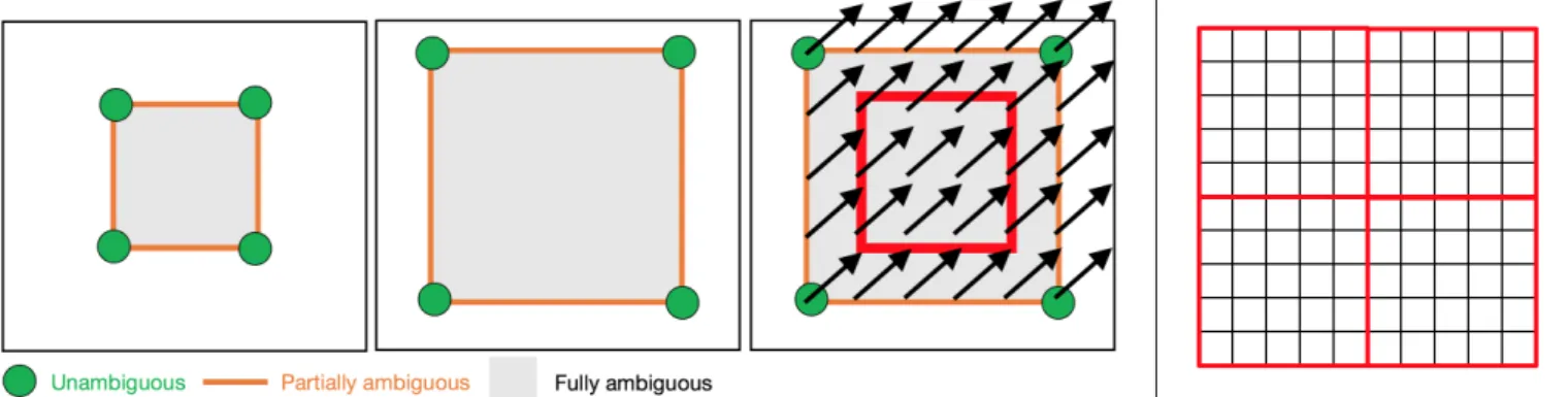
Figure 1: Left: The LDDMM momentum parameterization is ideal for patch-based prediction of image registrations. Consider registering a small square (left) to a large square (middle) with uniform intensity. Only the corner points suggest clear spatial
correspondences. Edges also suggest spatial correspondences, however, correspondences betweenindividualpoints on edges remain
ambiguous. Lastly, points interior to the squares have ambiguous spatial correspondences, which are established purely based on regularization. Hence, predicting velocity or displacement fields (which are spatially dense) from patches is challenging in these interior areas (right), in the absence of sufficient spatial context. Predicting a displacement field as illustrated in the right image from an interior patch (illustrated by the red square) would be impossible if both the target and the source image patches are uniform in intensity. In this scenario, the patch information would not provide sufficient spatial context to capture aspects of the
deformation. On the other hand, we know from LDDMM theory that the optimal momentum,m, to match images can be written
as m(x, t) =λ(x, t)∇I(x, t), where λ(x, t) 7→ Ris a spatio-temporal scalar field andI(x, t) is the image at timet [45, 19,17].
Hence, in spatially uniform areas (where correspondences are ambiguous)∇I= 0 and consequentiallym(x, t) = 0. This is highly
beneficial for prediction as the momentum only needs to be predicted at image edges. Right: Furthermore, as the momentum
is not spatially smooth, the regression approach does not need to account for spatial smoothness, which allows predictions with non-overlapping or hardly-overlapping patches as illustrated in the figure by the red squares. This is not easily possible for the prediction of displacement or velocity fields since these are expected to be spatially dense and smooth, which would need to be considered in the prediction. Consequentially, predictions of velocity or displacement fields will inevitably result in discontinuities across patch boundaries (i.e., across the red square boundaries shown in the figure) if they are predicted independently of each other.
the initial momenta for the test image pairs, and gener-ate the predicted deformation result simply by performing LDDMM shooting.
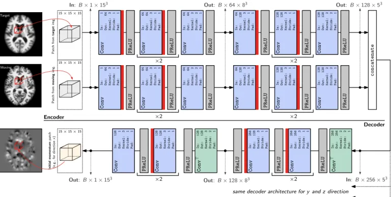
Fig.2shows the structure of the initial momentum pre-diction network. We first discuss the deterministic version of the network without dropout layers. We then introduce the Bayesian version of our network where dropout layers are used to convert the architecture into a probabilistic deep network. Finally, we discuss our strategy for patch pruning to reduce the number of patches needed for whole image prediction.
2.2.1. Deterministic network
Our goal is to learn a prediction function that takes two input patches, extracted at the same location6 from
the moving and target image, and predicts a desired
ini-tial vector-valued momentum patch, separated into thex, y andzdimensions, respectively. This prediction function should be learned from a set of training sample patches. These initial vector-valued momentum patches are obtained by numerical optimization of the LDDMM shooting formu-lation. More formally, given a 3D patch of size p×p×p voxels, we want to learn a functionf :R3p×R3p →R9p.
6The locations of these patches are the same locations with
re-spect to image grid coordinates, as the images are still unregistered at this point.
In our formulation,f is implemented by a deep neural net-work. Ideally, for two 3D image patches (u,v) =x0, with
u,v∈R3p, we wanty0 =f(x0) to be as close as possible to the desired LDDMM optimization momentum patchy
with respect to an appropriate loss function (e.g., the 1-norm). Our proposed architecture (forf) consists of two parts: anencoder and adecoder which we describe next.
Encoder. TheEncoderconsists of two parallel encoders which learn features from the moving/target image patches independently. Each encoder contains two blocks of three 3×3×3 3D convolution layers and PReLU [52] activation layers, followed by another 2×2×2 convolution+PReLU with a stride of two, cf. Fig. 2. The convolution layers with a stride of two reduce the size of the output patch, and essentially perform pooling operations. PReLU is an extension of the ReLU activation [53], given as
PReLU(x) = (
x, ifx >0
ax, otherwise ,
×2
Out: B×64×83
In: 64 Out: 64 Kernel: 3 Stride: 1 Pad: 1 Conv In: 1 Out: 64 Kernel: 3 Stride: 1 Pad: 1 Conv In: 64 Out: 64 Kernel: 2 Stride: 2 Pad: 1 Conv ×2 In: 128 Out: 128 Kernel: 3 Stride: 1 Pad: 1 Conv In: 64 Out: 128 Kernel: 3 Stride: 1 Pad: 1 Conv In: 128 Out: 128 Kernel: 2 Stride: 2 Pad: 1 Conv
Out:B×128×53 In:B×1×153
PReLU PReLU PReLU PReLU PReLU PReLU
In: 256 Out: 256 Kernel: 2 Stride: 2 Pad: 1 Conv > PReLU PReLU In: 256 Out: 256 Kernel: 3 Stride: 1 Pad: 1 Conv PReLU In: 256 Out: 128 Kernel: 3 Stride: 1 Pad: 1 Conv ×2 In: 128 Out: 128 Kernel: 3 Stride: 2 Pad: 1 Conv > PReLU PReLU In: 128 Out: 128 Kernel: 3 Stride: 1 Pad: 1 Conv In: 128 Out: 1 Kernel: 3 Stride: 1 Pad: 1 Conv ×2 ×2 In: 64 Out: 64 Kernel: 3 Stride: 1 Pad: 1 Conv In: 1 Out: 64 Kernel: 3 Stride: 1 Pad: 1 Conv In: 64 Out: 64 Kernel: 2 Stride: 2 Pad: 1 Conv ×2 In: 128 Out: 128 Kernel: 3 Stride: 1 Pad: 1 Conv In: 64 Out: 128 Kernel: 3 Stride: 1 Pad: 1 Conv In: 128 Out: 128 Kernel: 2 Stride: 2 Pad: 1 Conv
PReLU PReLU PReLU PReLU PReLU PReLU
concatenate P atch from ta rget img. P atch from moving img. Initial momentum patch (e.g., fo r direction x ) Encoder Decoder Target Moving
same decoder architecture for y and z direction
15×15×15
15×15×15
15×15×15 Target
Moving Target
Moving
In: B×256×53 Out: B×128×83
Out:B×1×153
Figure 2: 3D (probabilistic) network architecture. The network takes two 3D patches from the moving and target image as the
input, and outputs 3 3D initial momentum patches (one for each of the x, yandz dimensions respectively; for readability, only
one decoder branch is shown in the figure). In case of the deterministic network, see Sec.2.2.1, the dropout layers, illustrated by
, are removed. Conv: 3D convolution layer. Conv|: 3D transposed convolution layer. Parameters for theConvandConv|layers:
In: input channel. Out: output channel. Kernel: 3D filter kernel size in each dimension. Stride: stride for the 3D convolution.
Pad: zero-padding added to the boundaries of the input patch. Note that in this illustrationBdenotes the batch size.
Decoder. Each decoder’s structure is the inverse of the encoder, except that the number of features is doubled (256 in the first block and 128 in the second block) as the decoder’s input is obtained from thetwoencoder branches. We use 3D transposed convolution layers [54] with a stride of 2, which are shown as the cyan layers in Fig. 2and can be regarded as the backward propagation of 3D convolu-tion operaconvolu-tions, to perform “unpooling”. We also omit the non-linearity after the final convolution layer, cf. Fig.2.
The idea of using convolution and transpose of convo-lution to learn the pooling/unpooling operation is moti-vated by [55], and it is especially suited for our network as the two encoders perform pooling independently which prevents us from using the pooling index for unpooling in the decoder. During training, we use the 1-norm be-tween the predicted and the desired momentum to mea-sure the prediction error. We chose the 1-norm instead of the 2-norm as our loss function to be able to tolerate outliers and to generate sharper momentum predictions. Ultimately, we are interested in predicting the deforma-tion map and not the patch-wise momentum. However, this would require forming the entire momentum image from a collection of patches followed by shooting as part of the network training. Instead, predicting the momen-tum itself patch-wise significantly simplifies the network training procedure. Also note that, while we predict the
momentum patch-by-patch, smoothing is performed over the full momentum image (reassembled from the patches) based on the smoothing kernel, K, of LDDMM. Specifi-cally, when predicting the deformation parameters for the whole image, we follow a sliding window strategy to pre-dict the initial momentum in a patch-by-patch manner and then average the overlapping areas of the patches to obtain the final prediction result.
The number of 3D filters used in the network is 975,360. The overall number of parameters is 21,826,344. While this is a large number of parameters, we also have a very large number of training patches. For example, in our image-to-image registration experiments (see Sec.3), the total number of 15×15×15 3D training patches to train the prediction network is 1,002,404. This amounts to ap-proximately 3.4 billion voxels and is much larger than the total number of parameters in the network. Moreover, re-cent research [56] suggests that the degrees of freedom for a deep network can be significantly smaller than the number of its parameters.
exper-iments, such a combined network easily got stuck in poor local minima. As to the encoders, experiments do not show an obvious difference in prediction accuracy between using two independent encoders and one single large en-coder. However, such a two-encoder strategy is beneficial when extending the approach to multi-modal image reg-istration [36]. Hence, using a two-encoder strategy here will make the approach easily retrainable for multi-modal image registration. In short, our network structure can be viewed as a multi-input multi-task network, where each encoder learns features for one patch source, and each de-coder uses the shared image features from the ende-coders to predict one spatial dimension of the initial momenta. We remark that, if one were to predict the scalar-valued mo-mentum, λ, instead of the vector-valued momentum, m, the network architecture could remain largely unchanged. The main difference would be that only one decoder would be required. Due to the simpler network architecture such an approach could potentially speed-up predictions. How-ever, it remains to be investigated how such a network would perform in practice as the vector-valued momentum has been found to numerically better behave for LDDMM optimizations [50].
2.2.2. Probabilistic network
We extend our architecture to a probabilistic network using dropout [57], which can be viewed as (Bernoulli) ap-proximate inference in Bayesian neural networks [58, 59]. In the following, we briefly review the basic concepts, but refer the interested reader to the corresponding references for further technical details.
In our problem setting, we are given training patch tuplesxi= (ui,vi) with associated desired initial
momen-tum patches yi. We denote the collection of this train-ing data byX andY. In the standard, non-probabilistic setting, we aim for predictions of the form y0 = f(x0), given a new input patch x0, where f is implemented by the proposed encoder-decoder network. In the probabilis-tic setting, however, the goal is to make predictions of the form p(y0|x0,X,Y). As this predictive distribution is in-tractable for most underlying models (as it would require integrating over all possible models, and neural networks in particular), the idea is to condition the model on a set of random variables w. In case of (convolutional) neural networks with N layers, these random variables are the weight matrices, i.e., w = (Wi)Ni=1. However, evaluation of the predictive distribution p(y0|x0,X,Y) then requires the posterior over the weights p(w|X,Y) which can (usu-ally) not be evaluated analytically. Therefore, in varia-tional inference,p(w|X,Y) is replaced by a tractable vari-ational distributionq(w) and one minimizes the Kullback-Leibler divergence between q(w) andp(w|X, Y) with re-spect to the variational parameters w. This turns out to be equivalent to maximization of the log evidence lower
bound (ELBO). When the variational distribution is
de-fined as
q(Wi) =Mi·diag([zi,j]jK=1i ), zi,j ∼Bernoulli(d) , (5)
whereMiis the convolutional weight,i= 1, . . . , N,dis the
probability thatzi,j= 0 andKiis chosen appropriately to
match the dimensionality ofMi, Gal et al. [58] show that ELBO maximization is achieved by training with dropout [57]. In the case of convolutional neural networks, dropout is applied after each convolution layer (with dropout prob-ability d)7. In Eq. (5), Mi is the variational parame-ter which is optimized during training. Evaluation of the predictive distributionp(y0|x0,X,Y) can then be approx-imated via Monte-Carlo integration, i.e.,
p(y0|x0,X,Y)≈ 1 T
T
X
t=1 ˆ
f(x0,wˆ) . (6)
In detail, this corresponds to averaging the output of T forward passes through the network with dropoutenabled. Note that ˆf and ˆw now correspond to random variables, as dropout means that we sample, in each forward pass, which connections are dropped. In our implementation, we add dropout layers after all convolutional layers except for those used as pooling/unpooling layers (which are con-sidered non-linearities applied to the weight matrices [58]), as well as the final convolution layer in the decoder, which generates the predicted momentum. We train the network using stochastic gradient descent (SGD).
Network evaluation. For testing, we keep the dropout layers enabled to maintain the probabilistic property of the network, and sample the network to obtain multiple momentum predictions for one moving/target image pair. We then choose the sample mean as the prediction result, see Eq. (6), and perform LDDMM shooting using all the samples to generate multiple deformation fields. The lo-cal variance of these deformation fields can then be used as an uncertainty estimate of the predicted deformation field. When selecting the dropout probability, d, a prob-ability of 0.5 would provide the largest variance, but may also enforce too much regularity for a convolutional net-work, especially in our case where dropout layers are added after every convolution layer. In our experiments, we use a dropout probability of 0.2 (for all dropout units) as a balanced choice.
2.2.3. Patch pruning
As discussed in Sec.2.2.1, we use a sliding-window ap-proach to predict the deformation parameters (the mo-menta forQuicksilver) patch-by-patch for a whole image. Thus, computation time is proportional to the number of the patches we need to predict. When using a 1-voxel slid-ing window stride, the number of patches to predict for a
7with additionall
2regularization on the weight matrices of each
Prediction net
w
ork
P
atch
extraction
T ◦Φ
Co
rrection
net
w
ork
P
atch
extraction
+
Initial momenta prediction(trained first)
applybackward warp Φ
Moving (M)
T
arget (T)
Initial momenta
Correction momenta
Final momenta Correction momenta prediction(trained second)
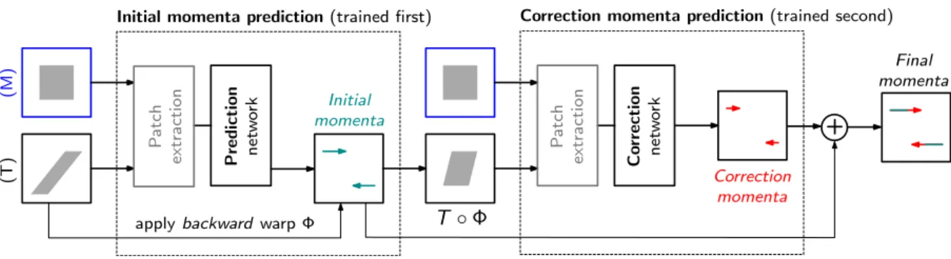
Figure 3: The full prediction + correction architecture for LDDMM momenta. First, a rough prediction of the initial momentum,
mLP, is obtained by the prediction network (LP) based on the patches from the unaligned moving image,M and target image,
T, respectively. The resulting deformation maps Φ−1 and Φ are computed by shooting. Φ is then applied to the target image to
warp it to the space of the moving image. A second correction network is then applied to patches from the moving imageM and
the warped target imageT◦Φ to predict a correction of the initial momentum,mC in the space of the moving image, M. The
final momentum is then simply the sum of the predicted momenta,m=mLP+mC, which parameterizes a geodesic between the
moving image and the target image.
whole image could be substantial. For a typical 3D im-age of size 128×128×128 using a 15×15×15 patch for prediction will require more than 1.4 million patch predic-tions. Hence, we use two techniques to drastically reduce the number of patches needed for deformation prediction. First, we perform patch pruning by ignoring all patches that belong to the background of both the moving image and the target image. This is justified, because accord-ing to LDDMM theory the initial momentum in constant image regions, and hence also in the image background, should be zero. Second, we use a large voxel stride (e.g., 14 for 15×15×15 patches) for the sliding window oper-ations. This is reasonable for our initial momentum pa-rameterization because of the compact support (at edges) of the initial momentum and the spatial shift invariance we obtain via the pooling/unpooling operations. By us-ing these two techniques, we can reduce the number of predicted patches for one single image dramatically. For example, by 99.995% for 3D brain images of dimension 229×193×193.
2.3. Correction network
There are two main shortcomings of the deformation prediction network. (i) The complete iterative numeri-cal approach typinumeri-cally used for LDDMM registration is replaced by asingleprediction step. Hence, it is not possi-ble to recover from any prediction errors. (ii) To facilitate training a network with a small number of images, to make predictions easily parallelizable, and to be able to perform predictions for large 3D image volumes, the prediction net-work predicts the initial momentumpatch-by-patch. How-ever, since patches are extracted at the same spatial grid locations from the moving and target images, large defor-mations may result in drastic appearance changes between a source and a target patch. In the extreme case, corre-sponding image information may no longer be found for a given source and target patch pair. This may happen, for
example, when a small patch-size encounters a large defor-mation. While using larger patches would be an option (in the extreme case the entire image would be represented by one patch), this would require a network with substantially larger capacity (to store the information for larger image patches and all meaningful deformations) and would also likely require much larger training datasets8.
To address these shortcomings, we propose a two-step prediction approach to improve overall prediction accu-racy. The first step is our already described prediction network. We refer to the second step as the correction
network. The task of the correction network is to
com-pensate for prediction errors of the first prediction step. The idea is grounded in two observations: The first ob-servation is that patch-based prediction is accurate when the deformation inside the patch is small. This is sen-sible as the initial momentum is concentrated along the edges, small deformations are commonly seen in training images, and less deformation results in less drastic mo-mentum values. Hence, more accurate predictions are ex-pected for smaller deformations. Our second observation is that, given the initial momentum, we are able to gen-erate the whole geodesic path using the geodesic shooting equations. Hence, we can generate two deformation maps: the forward warp Φ−1 that maps the moving image to the coordinates of the target image, and the backward warp Φ mapping the target image back to the coordinates of the moving image. Hence, after the first prediction step us-ing our prediction network, we can warp the target image back to the moving imageM viaT◦Φ. We can then train
thecorrection networkbased on the difference between the
moving imageM and the warped-back target imageT◦Φ,
8In fact, we have successfully trained prediction models with as
such that it makes adjustments to the initial momentum predicted in the first step by our prediction network. Be-causeM andT◦Φ are in the same coordinate system, the differences between these two images are small as long as the predicted deformation is reasonable, and more accu-rate predictions can be expected. Furthermore, the cor-rection for the initial momentum is then performed in the original coordinate space (of the moving image) which al-lows us to obtain an overall corrected initial momentum, m0. This is for example a useful property when the goal is to do statistics with respect to a fixed coordinate system, for example, an atlas coordinate system.
Fig. 3 shows a graphical illustration of the resulting two-step prediction framework. In the framework, the cor-rection network has the same structure as the prediction network, and the only difference is the input of the net-works and the output they produce. Training the overall framework is done sequentially:
1. Train the prediction network using training images and the ground truth initial momentum obtained by numerical optimization of the LDDMM registration model.
2. Use the predicted momentum from the prediction network to generate deformation fields to warp the target images in the training dataset back to the space of the moving images.
3. Use the moving images and the warped-back target images to train the correction network. The correc-tion network learns to predict thedifferencebetween the ground truth momentum and the predicted mo-mentum from the prediction network.
Using the framework during testing is similar to the train-ing procedure, except here the outputs from the predic-tion network (using moving and target images as input) and the correction network (using moving and warped-back target images as input) are summed up to obtain the final predicted initial momentum. This summation is justified from the LDDMM theory as it is performed in a fixed coordinate system (a fixed tangent space), which is the coordinate system of the moving image. Experiments show that our prediction+correction approach results in lower training and testing error compared with only using a prediction network, as shown in Sec.2.4and Sec.3.
2.4. Datasets / Setup
We evaluate our method using three 3D brain image registration experiments. The first experiment is designed to assess atlas-to-image registration. In this experiment, the moving image is always the atlas image. The second experiment addresses generalimage-to-imageregistration. The final experiment exploresmulti-modal image registra-tion; specifically, the registration of T1-weighted (T1w) and T2-weighted (T2w) magnetic resonance images.
For the atlas-to-imageregistration experiment, we use 3D image volumes from the OASIS longitudinal dataset [60]. Specifically, we use the first scan of all subjects, resulting in 150 brain images. We select the first 100 images as our training target images and the remaining 50 as our test target images. We create an unbiased atlas [61] from all training data usingPyCA9[50,62], and use the atlas as the moving image. We use the LDDMM shooting algorithm to register the atlas image to all 150 OASIS images. The obtained initial momenta from the training data are used to train our network; the remaining momenta are used for validation.
For theimage-to-imageregistration experiment, we use all 373 images from the OASIS longitudinal dataset as the training data, and randomly select target images from dif-ferent subjects for every image, creating 373 registrations for the training of our prediction and correction networks. For testing, we choose the four datasets (LPBA40,IBSR18, MGH10, CUMC12) evaluated in [33]. We perform LDDMM shooting for all training registrations, and follow the eval-uation procedure described in [33] to perform pairwise reg-istrations within all datasets, resulting in a total of 2168 registration (1560 fromLPBA40, 306 fromIBSR18, 90 from MGH10, 132 fromCUMC12) test cases.
For the multi-modal registration experiment, we use the IBIS 3D Autism Brain image dataset [34]. This dataset contains 375 T1w/T2w brain images from 2 years old sub-jects. We select 359 of the images for training and use the remaining 16 images for testing. For training, we ran-domly select T1w-T1w image pairs and perform LDDMM shooting to generate the optimization momenta. We then train the prediction and correction networks to predict the momenta obtained from LDDMM T1w-T1w optimization using the image patches from the corresponding T1w
mov-ing image and T2w target image as network inputs. For
testing, we perform pair-wise T1w-T2w registrations for all 16 test images, resulting in 250 test cases. For comparison, we also train a T1w-T1w prediction+correction network that performs prediction on the T1w-T1w test cases. This network acts as the “upper-bound” of the potential perfor-mance of our multi-modal networks as it addresses the uni-modal registration case and hence operates on image pairs which have very similar appearance. Furthermore, to test prediction performance when using very limited training data, we also train a multi-modal prediction network and a multi-modal prediction+correction network using only 10 of the 365 training images which are randomly chosen for training. In particular, we perform pair-wise T1w-T1w registration on the 10 images, resulting in 90 registration pairs. We then use these 90 registration cases to train the multi-modal prediction networks.
For skull stripping, we use FreeSurfer [63] for the OA-SIS dataset and AutoSeg [64] for the IBIS dataset. The
Epoch L1
loss per patch
1 1.5 2 2.5 3
3.5 Predict, 1-20 epoch
Correct, 1-20 epoch Predict, 21-40 epoch
0 10 20 30 40
(a) Atlas-to-Image
Epoch L1
loss per patch
4 6 8 10 12 14 16
18 Predict, 1-10 epoch
Correct, 1-10 epoch Predict, 11-20 epoch
0 5 10 15 20
(b)Image-to-Image
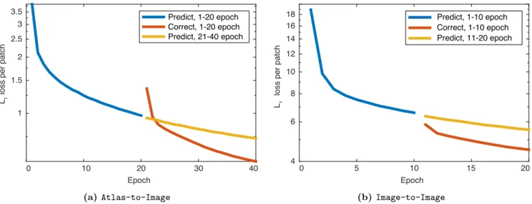
Figure 4: Log10plot ofl1 training loss per patch. The loss is averaged across all iterations for every epoch for both the
Atlas-to-Image case and the Image-Atlas-to-Image case. The combined prediction + correction networks obtain a lower loss per patch than the loss obtained by simply training the prediction networks for more epochs.
4 evaluation datasets for image-to-image experiment are already skull stripped as described in [33]. All images used in our experiments are first affinely registered to the ICBM MNI152 nonlinear atlas [65] using NiftyReg10 and intensity normalized via histogram equalization prior to atlas building and LDDMM registration. All 3D volumes are of size 229×193×193 except for the LPBA dataset (229×193×229), where we add additional blank image voxels for the atlas to keep the cerebellum structure. LD-DMM registration is done using PyCA11 [50] with SSD as the image similarity measure. We set the parameters for the regularizer of LDDMM12 to L=
−a∇2
−b∇(∇·) +c as [a, b, c] = [0.01,0.01,0.001], and σ in Eqn. 3 to 0.2. We use a 15×15×15 patch size for deformation pre-diction in all cases, and use a sliding window with step-size 14 to extract patches for training. The only excep-tion is for the multi-modal network which is trained us-ing only 10 images, where we choose a step-size of 10 to generate more training patches. Note that using a stride of 14 during training means that we are in fact discard-ing available traindiscard-ing patches to allow for reasonable net-work training times. However, we still retain a very large number of patches for training. To check that our num-ber of patches for training is sufficient, we performed ad-ditional experiments for the image-to-image registration
10https://cmiclab.cs.ucl.ac.uk/mmodat/niftyreg
11https://bitbucket.org/scicompanat/pyca
12This regularizer is too weak to assure a diffeomorphic
transfor-mation based on thesufficientregularity conditions discussed in [13]. For these conditions to hold in 3D, Lwould need to be at least a differential operator of order 6. However, as long as the obtained velocity fieldsvare finite over the unit interval, i.e.,R1
0 kvk2Ldt <∞
for an Lof at least order 6, we will obtain a diffeomorphic trans-form [51]. In the discrete setting, this condition will be fulfilled for finite velocity fields. To side-step this issue, models based on Gaus-sian or multi-GausGaus-sian kernels [66] could also be used instead.
task using smaller strides when selecting training patches. Specifically, we doubled and tripled the training size for the prediction network. These experiments indicated that increasing the training data size further only results in marginal improvements, which are clearly outperformed by a combined prediction + correction strategy. Explor-ing alternative network structures, which may be able to utilize larger training datasets, is beyond the scope of this paper, but would be an interesting topic for future re-search.
The network is implemented in PyTorch13, and opti-mized using Adam[67]. We set the learning rate to 0.0001 and keep the remaining parameters at their default val-ues. We train the prediction network for 10 epochs for the image-to-image registration experiment and the multi-modal image registration experiment, and 20 epochs for the atlas-to-image experiment. The correction networks are trained using the same number of epochs as their cor-responding prediction networks. Fig.4shows thel1 train-ing loss per patch averaged for every epoch for the atlas-to-image and the image-atlas-to-image experiments. For both, using a correction network in conjunction with a predic-tion network results in lower training error compared with training the prediction network for more epochs.
3. Results
3.1. Atlas-to-Image registration
For the atlas-to-image registration experiment, we test two different sliding window strides for our patch-based prediction method: stride = 5 and stride = 14. We trained additional prediction networks predicting the initial veloc-ity v0 = Km0 and the displacement field Φ(1)−id of
Deformation Error for each voxel[mm] detJ >0
Data percentile for all voxels 0.3% 5% 25% 50% 75% 95% 99.7%
Affine 0.0613 0.2520 0.6896 1.1911 1.8743 3.1413 5.3661 N/A D, velocity, stride 5 0.0237 0.0709 0.1601 0.2626 0.4117 0.7336 1.5166 100% D, velocity, stride 14 0.0254 0.075 0.1675 0.2703 0.415 0.743 1.5598 100% D, deformation, stride 5 0.0223 0.0665 0.1549 0.2614 0.4119 0.7388 1.5845 56% D, deformation, stride 14 0.0242 0.0721 0.1671 0.2772 0.4337 0.7932 1.6805 0%
P, momentum, stride 14, 50 samples 0.0166 0.0479 0.1054 0.1678 0.2546 0.4537 1.1049 100% D, momentum, stride 5 0.0129 0.0376 0.0884 0.1534 0.2506 0.4716 1.1095 100% D, momentum, stride 14 0.013 0.0372 0.0834 0.1359 0.2112 0.3902 0.9433 100% D, momentum, stride 14, 40 epochs 0.0119 0.0351 0.0793 0.1309 0.2070 0.3924 0.9542 100% D, momentum, stride 14 + correction 0.0104 0.0309 0.0704 0.1167 0.185 0.3478 0.841 100%
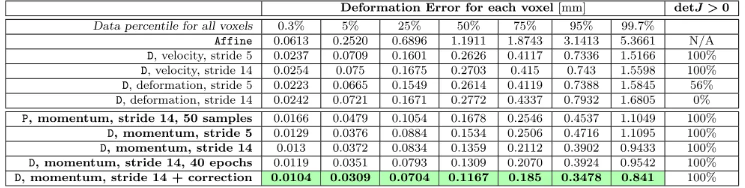
Table 1: Test result foratlas-to-image registration. The table shows the distribution of the 2-norm of the deformation error of
the predicted deformation with respect to the deformation obtained by numerical optimization. Percentiles of the displacement errors are shown to provide a complete picture of the error distribution over just reporting the mean or median errors over all
voxels within the brain mask in the dataset. D: deterministic network;P: probabilistic network; stride: stride length of the sliding
window for whole image prediction; velocity: predicting initial velocity; deformation: predicting the deformation field; momentum:
predicting the initial momentum; correction: using the correction network. ThedetJ >0column shows the ratio of test cases
with only positive-definite determinants of the Jacobian of the deformation map to the overall number of registrations (100%
indicates that all registration results were diffeomorphic). Our initial momentum networks are highlighted in bold. The best
results are also highlighted inbold.
LDDMM to show the effect of different deformation pa-rameterizations on deformation prediction accuracy. We generate the predicted deformation map by integrating the shooting equation4for the initial momentum and the ini-tial velocity parameterization respectively. For the dis-placement parameterization we can directly read-off the map from the network output. We quantify the deforma-tion errors per voxel using the voxel-wise two-norm of the deformation error with respect to the result obtained via numerical optimization for LDDMM using PyCA. Table 1 shows the error percentiles over all voxels and test cases.
We observe that the initial momentum network has better prediction accuracy compared to the results ob-tained via the initial velocity and displacement parame-terization in both the 5-stride and 14-stride cases. This validates our hypothesis that momentum-based LDDMM is better suited for patch-wise deformation prediction. We also observe that the momentum prediction result using a smaller sliding window stride is slightly worse than the one using a stride of 14. This is likely the case, because in the atlas-to-image setting, the number of atlas patches that extract features from the atlas image is very limited, and using a stride of 14 during the training phase further reduces the available data from the atlas image. Thus, during testing, the encoder will perform very well for the 14-stride test cases since it has already seen all the in-put atlas patches during training. For a stride of 5 how-ever, unseen atlas patches will be input to the network, resulting in reduced registration accuracy14. In contrast, the velocity and the displacement parameterizations result
14This behavior could likely be avoided by randomly sampling
patch locations during training instead of using a regular grid. How-ever, since we aim at reducing the number of predicted patches we did not explore this option and instead maintained the regular grid sampling.
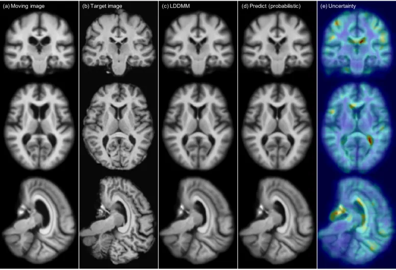
(a) Moving image (b) Target image (c) LDDMM (d) Predict (probabilistic) (e) Uncertainty
Figure 5: Atlas-to-image registration example. Fromlefttoright: (a): moving (atlas) image; (b): target image; (c): deformation
from optimizing LDDMM energy; (d): deformation from using the mean of 50 samples from the probabilistic network with
stride=14 and patch pruning; (e): the uncertainty map as square root of the sum of the variances of the deformation in x,y,
and z directions mapped onto the predicted deformation result. The coloring indicates the level of uncertainty, withred = high
uncertaintyandblue = low uncertainty. Best-viewed in color.
Fig. 5 shows one example atlas-to-image registration case. The predicted deformation result is very similar to the deformation from LDDMM optimization. We compute the square root of the sum of the variance of the deforma-tion in the x, y and z directions to quantify deformation uncertainty, and visualize it on the rightmost column of the figure. The uncertainty map shows high uncertainty along the ventricle areas where drastic deformations occur, as shown in the moving and target images.
3.2. Image-to-Image registration
In this experiment, we use a sliding window stride of 14 for both the prediction network and the correction network during evaluation. We mainly compare the fol-lowing three LDDMM-based -methods: (i) the numerical LDDMM optimization approach (LO) as implemented in PyCA, which acts as an upper bound on the performance of our prediction methods; and two flavors of Quicksilver: (ii) only the prediction network (LP) and (iii) the predic-tion+correction network (LPC). Example registration cases
are shown in Fig. 9.
3.2.1. LDDMM energy
0 0.2 0.4 0.6 0.8
FLIRT AIR ANIMAL ART Demons FNIRT Fluid SICLE SyN SPM5N8 SPM5N SPM5U SPM5D LO LP LPC LPC2 LPC3 LPP Dataset: LBPA40
0 0.2 0.4 0.6 0.8
FLIRT AIR ANIMAL ART Demons FNIRT Fluid SICLE SyN SPM5N8 SPM5N SPM5U SPM5D
LO LP LPC
LPC2 LPC3 LPP
Dataset: ISBR18
0 0.2 0.4 0.6 0.8
FLIRT AIR ANIMAL ART Demons FNIRT Fluid SICLE SyN SPM5N8 SPM5N SPM5U SPM5D LO LP LPC LPC2 LPC3 LPP Dataset: CUMC12
0 0.2 0.4 0.6 0.8
FLIRT AIR ANIMAL ART Demons FNIRT Fluid SICLE SyN SPM5N8 SPM5N SPM5U SPM5D LO LP LPC LPC2 LPC3 LPP
Dataset: MGH10
Figure 6: Overlap by registration method for theimage-to-image registration case. The boxplots illustrate the mean target
overlap measures averaged over all subjects in each label set, where mean target overlap is the average of the fraction of the target region overlapping with the registered moving region over all labels. The proposed LDDMM-based methods in this paper
are highlighted in red. LO= LDDMM optimization; LP = prediction network;LPC = prediction network + correction network.
LPP: prediction network + using the prediction network for correction. LPC2/LPC3: prediction network + iteratively using the
correction network 2/3 times. Horizontal red lines show theLPCperformance in the lower quartile to upper quartile (best-viewed
in color). The medians of the overlapping scores for [LPBA40,IBSR18,CUMC12, MGH10] forLO,LPand LPC are: LO: [0.702, 0.537,
0.536, 0.563];LP: [0.696, 0.518, 0.515, 0.549];LPC: [0.702, 0.533, 0.526, 0.559]. Best-viewed in color.
achievable by training dataset specific models. Table 2 shows the results for the four test datasets. Compared with the initial LDDMM energy based on affine registra-tion to the atlas space in theinitialcolumn, bothLPand LPChave drastically lower LDDMM energy values; further, these values are only slightly higher than those for LO. Furthermore, compared with LP, LPCgenerates LDDMM energy values that are closer to LO, which indicates that using the prediction+correction approach results in mo-menta which are closer to the optimal solution than the ones obtained by using the prediction network only.
3.2.2. Label overlap
For image-to-image registration we follow the approach in [33] and calculate the target overlap (TO) of labeled brain regions after registration: T O = |lm∩lt|
|lt| , where lm
and lt indicate the corresponding labels for the moving
LDDMM energyfor image-to-image test datasets LPBA40
initial LO LP LPC
0.120±0.013 0.027±0.004 0.036±0.005 0.030±0.005 IBSR18
initial LO LP LPC
0.214±0.032 0.037±0.008 0.058±0.013 0.047±0.011 CUMC12
initial LO LP LPC
0.246±0.015 0.044±0.003 0.071±0.004 0.056±0.004 MGH10
initial LO LP LPC
0.217±0.012 0.039±0.003 0.062±0.004 0.049±0.003
Table 2: Mean and standard deviation of the LDDMM energy
for four image-to-image test datasets. initial: the initial
LD-DMM energy between the original moving image and the target image after affine registration to the atlas space, i.e. the
orig-inal image matching energy. LO: LDDMM optimization. LP:
prediction network. LPC: prediction+correction network.
correction network are identical, and whether the predic-tion network can be used in the correcpredic-tion step. Another question is if the correction network can be applied multi-ple times in the correction step to further improve results. Thus, to test the usefulness of the correction network in greater depth, we also create three additional formulations of our prediction framework: (i) prediction network + us-ing the same prediction network to replace the correction network in the correction step (LPP); (ii) applying the cor-rection network twice (LPC2) and (iii) applying the correc-tion network three times (LPC3).
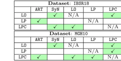
Fig. 6 shows the evaluation results. Several points should be noted: first, the LDDMM optimization perfor-mance is on par with SyN [68], ART [69] and the SPM5 DARTEL Toolbox (SPM5D) [70]. This is reasonable as these methods are all non-parametric diffeomorphic or home-omorphic registration methods, allowing the modeling of large deformations between image pairs. Second, using only the prediction network results in a slight performance drop compared to the numerical optimization results (LO), but the result is still competitive with the top-performing registration methods. Furthermore, also using the cor-rection network boosts the deformation accuracy nearly to the same level as the LDDMM optimization approach (LO). The red horizontal lines in Fig.6show the lower and upper quartiles of the target overlap score of the predic-tion+correction method. Compared with other methods, our prediction+correction network achieves top-tier per-formance for label matching accuracy at a small fraction of the computational cost. Lastly, in contrast to many of the other methods Quicksilver produces virtually no outliers. One can speculate that this may be the benefit of learning to predict deformations from a largepopulationof data, which may result in a prediction model which con-servatively rejects unusual deformations. Note that such a population-based approach is very different from most
ex-isting registration methods which constrain deformations based on a regularizer chosen for a mathematical regis-tration model. Ultimately, a deformation model for image registration should model what deformations are expected. Our population-based approach is a step in this direction, but, of course, still depends on a chosen regularizer to gen-erate training data. Ideally, this regularizer itself should be learned from data.
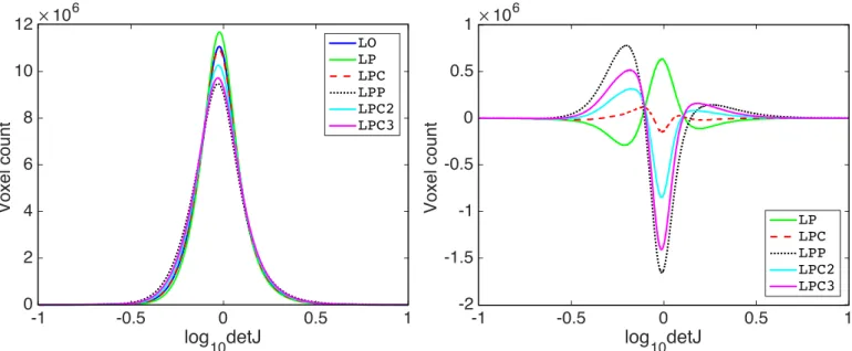
An interesting discovery is that LPP, LPC2 and LPC3 produce label overlapping scores that are on-par withLPC. However, as we will show in Sec.3.2.3,LPP,LPC2andLPC3 deviate from our goal of predicting deformations that are similar to the LDDMM optimization result (LO). In fact, they produce more drastic deformations that can lead to worse label overlap and even numerical stability problems. These problems can be observed in the LPBA40 results shown in Fig.6, which show more outliers with low over-lapping scores forLPPandLPC3. In fact, there are 12 cases for LPP where the predicted momentum cannot generate deformation fields via LDDMM shooting usingPyCA, due to problems related to numerical integration. These cases are therefore not included in Fig.6. PyCAuses an explicit Runge-Kutta method (RK4) for time-integration. Hence, numerical instability is likely due to the use of a fixed step size for this time-integration which is small enough for the deformations expected to occur for these brain registration tasks, but which may be too large for the more extreme momentaLPPandLPC3create for some of these cases. Us-ing a smaller step-size would regain numerical stability in this case.
To study the differences among registration algorithms
statistically, we performed pairedt-tests15with respect to
the target overlap scores between our LDDMM variants (LO,LP,LPC) and the methods in [33]. Our null-hypothesis is that the methods show the same target overlap scores. We use a significance level of α= 0.05/204 for rejection of this null-hypothesis. We also computed the mean and the standard deviation of pair-wise differences between our LDDMM variants and these other methods. Table3shows the results. We observe that direct numerical optimization of the shooting LDDMM formulation via PyCA (LO) is a highly competitive registration method and shows better target overlap scores than most of the other registration algorithms for all four datasets (LPBA40,IBSR18,CUMC12, andMGH10). Notable exceptions areART(onLPBA40),SyN (on LBPA40), and SPM5D (on IBSR18). However, perfor-mance decreases are generally very small: −0.017,−0.013, and −0.009 mean decrease in target overlap ratio for the three aforementioned exceptions, respectively. Specifically,
15To safe-guard against overly optimistic results due to

![Fig. 6 shows the evaluation results. Several points should be noted: first, the LDDMM optimization perfor-mance is on par with SyN [68], ART [69] and the SPM5 DARTEL Toolbox (SPM5D) [70]](https://thumb-us.123doks.com/thumbv2/123dok_us/8280342.2192857/15.892.60.436.132.330/evaluation-results-points-lddmm-optimization-perfor-dartel-toolbox.webp)