INTEGRAL-EQUATION-BASED FAST
ALGORITHMS AND GRAPH-THEORETIC
METHODS FOR LARGE-SCALE SIMULATIONS
Bo Zhang
A dissertation submitted to the faculty of the University of North Carolina at Chapel Hill in partial fulfillment of the requirements for the degree of Doctor of Philosophy in the Department of Mathematics.
Chapel Hill 2010
Approved by:
Professor Jingfang Huang Professor Michael L. Minion Professor Laura Miller Professor Nikos P. Pitsianis
c 2010 Bo Zhang
ABSTRACT
BO ZHANG: Integral-equation-based Fast Algorithms and Graph-theoretic Methods for Large-scale Simulations
(Under the direction of Professor Jingfang Huang)
ACKNOWLEGEMENTS
First and foremost, I would like to express my greatest gratitude and appreciation to my advisor Jingfang Huang, without whom this dissertation would simply be impossible. Huang has generously helped me and supported me in various ways. It is my great honor to have him as my advisor.
I thank Xiaobai Sun and Nikos Pitsianis for broaden my knowledge in the field of computer science, for providing me with unconditional help, support and guidance on many topics of this dissertation in the past one and a half years. The benefit of their suggestions could hardly be exaggerated.
I am very grateful to Michael Minion and Laura Miller, for their intelligent advice and helps during my study at UNC.
I would like to thank the support from my family. To my parents, for raising me, educating me, and loving me. To my wife Jianyu, for believing in me, supporting me, and encouraging me in all these years.
TABLE OF CONTENTS
LIST OF TABLES viii
LIST OF FIGURES ix
1 Introduction 1
2 Fast Multipole Method 8
2.1 Spatial Domain Adaptive Tree Structure . . . 12
2.2 Approximations and Translations . . . 17
2.3 Algorithm Structure of Adaptive FMM . . . 25
2.4 FMM-Yukawa in FMMsuite . . . 30
2.4.1 FMM-Yukawa Installation Instructions . . . 31
2.4.2 A Sample Driver File . . . 32
2.4.3 Test Run Description . . . 33
3 Parallelization of Fast Multipole Method on Multicore Architectures 37 3.1 Precursors of Parallel FMM . . . 38
3.2 Analytical Parallel FMM . . . 40
3.2.1 The Absolute Critical Path . . . 40
3.2.2 Maximum Concurrency under Dependency Constraints . . . 43
3.3 A Graph-Theoretic Parallelization Approach . . . 47
3.3.1 Parallelization Scheme for Upward Pass . . . 48
3.3.2 Parallelization Scheme for Downward Pass . . . 51
3.4 Numerical Experiments . . . 54
4 A Kernel Independent Fourier-series-based Fast Multipole Method 62 4.1 Precursors of Kernel-Independent FMM . . . 63
4.2 Kernel Approximation . . . 65
4.3 Translation Operators . . . 69
4.4 Algorithm Structure and Further Improvements . . . 78
4.5 Numerical Results . . . 89
LIST OF TABLES
2.1 Timing results for FMM-Yukawa for 3-digit accuracy with charges
uni-formly distributed inside the cube [−0.5,0.5]3 . . . . 34
2.2 Timing results for FMM-Yukawa for 6-digit accuracy with charges uni-formly distributed inside the cube [−0.5,0.5]3 . . . 35
2.3 Timing results for FMM-Yukawa for 3-digit accuracy with charges dis-tributed on the surface of a sphere . . . 35
2.4 Timing results for FMM-Yukawa for 6-digit accuracy with charges dis-tributed on the surface of a sphere . . . 35
3.1 Complexity analysis of parallel particle simulation . . . 41
3.2 CPU execution time VS number of threads . . . 57
3.3 Timing results for TM E operation at every level in Up direction . . . 58
3.4 CPU execution time VS N for uniform sampling . . . 61
3.5 CPU execution time VS N for nonuniform sampling . . . 61
4.1 Maximum approximation error for 1 x2: p= 10 and α = 2π 9 . . . 68
4.2 Half period expansion error . . . 72
4.5 Timing results of uniform FMM for 6-digit accuracy. Charges are dis-tributed in the unit square whose interactions are described by kernel 1 r2. Control relative error in kernel approximation. . . 92
4.6 Timing results of uniform FMM for 6-digit accuracy. Charges are dis-tributed in the unit square whose interactions are described by kernel 1 r2. Control absolute error in kernel approximation. . . 93
LIST OF FIGURES
1.1 Normal stress distribution (left) and its zoomed view (right) . . . 4
1.2 Parallel speedup vs. number of processors . . . 4
2.1 Box (b) and its associated lists 1 to 5 . . . 14
2.2 The U plist for the box (b) . . . 16
2.3 Screenshot of Fast Multipole Methods website . . . 31
2.4 Linear relationship between CPU time and N . . . 36
3.1 Exponential node growth rate . . . 42
3.2 Potential concurrency under dependence constraints . . . 44
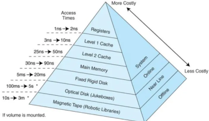
3.3 Memory hierarchy diagram . . . 46
3.4 Upward pass parallelization scheme . . . 50
3.5 Parallelization scheme forTM E & TEE operators . . . 53
3.6 CPU execution time VS number of threads . . . 57
3.7 CPU execution time VS N for uniform sampling . . . 59
3.8 CPU execution time VS N for nonuniform sampling . . . 60
4.1 Kernel approximation region . . . 66
4.2 (b) and two entries c1 and c2 of b’s list 3 . . . 84
4.3 Relative approximation error for kernel 1 r2 in the first quadrant . . . 92
4.4 Absolute approximation error for kernel 1 r2 in the first quadrant . . . 93
Chapter 1
Introduction
In the last two decades, the scientific community has witnessed the broad influence and impact of the seminal work by Greengard and Rokhlin in 1987 [34] on particle simula-tions using the fast multipole method (FMM). Due to its arithmeticO(N) orO(NlogN) complexity, in linear or super linear proportional to the numberN of interacting particles [34, 35], the FMM has accelerated or enabled many important large-scale calculations or simulations wherever directly applicable, in scientific and engineering studies. In partic-ular, the FMM has inspired the study of integral equation method as a new and effective approach for numerical solutions or simulations of different types of physical, chemical or biochemical processes that are traditionally modeled as boundary value problems of partial differential equations (see, for example, [59, 60, 55, 53, 54]).
The fundamental observation in the FMM is that the numerical rank of the far-field (“well-separated”) interactions is relatively low and hence can be “compressed” into p terms (depending on the required accuracy) of the so-called “multipole expansion”. For the Coulomb interactions, assuming R
ρi
> c0 > 1 for “source” i carrying a charge qi located at (ρi, αi, βi) in the spherical coordinate, the multipole expansion is given by
Φ(R, θ, φ) = N
X
i=1
qi· 1 |R−ρi|
≈ p
X
n=0
m=n
X
m=−n MnmY
m n (θ, φ)
Rn+1 (1.1)
Mnm = 8 N
X
i=1
qi·Yn−m(αi, βi). (1.2)
The spherical harmonic function of order n and degree m is defined according to the formula in [2].
Ynm(θ, φ) =
s
(2n+ 1)(n− |m|)! 4π(n+|m|)! ·P
|m|
n (cosθ)e
imφ, (1.3)
and Pm
n is the associated Legendre polynomial.
For arbitrary distributions of particles, a hierarchical oct-tree (in 3D) is generated so that each particle is associated with boxes at different levels. A divide-and-conquer strategy is applied to account for the far-field interactions at each level in the tree struc-ture, by accumulating information from the multipole expansions in the interaction list to the “local expansions” given by
Φ(R, θ, φ) = N
X
i=1
qi· 1 |R−ρi|
≈ p
X
n=0
m=n
X
m=−n
Lmn ·RnYnm(θ, φ) (1.4)
where {Lmn} are the local expansion coefficients. The local expansion of a parent box which collects its far-field contributions can be transmitted to its children. As each par-ticle only interacts with the box and nearby parpar-ticles at the finest level, and information at higher levels is transferred using a combination of multipole and local expansions, the original FMM has asymptotically optimal complexity O(N). However, because the multipole-to-local translation requires prohibitive 189p4 operations for each box, the huge
was reduced from 189p4 to 40p2 + 6p3 for each box. Numerical experiments show that
the new-version FMM breaks even with direct calculation when the number of particles N = 750 for three digit accuracy, and N = 1500 for six digit accuracy for the Coulomb interactions. The details of the FMM will be discussed in Chpater 2.
The new-version FMM poses multiple challenges on software or hardware implemen-tations, and presents a fundamental question on computer system support of large-scale simulation in terms of software and hardware design and development. Despite the chal-lenges, a lot of efforts have been devoted to developing new-version FMM-based numerical tools, in order to meet the increasing and practical demand in computational sciences and engineering. In the following, we discuss three recent research efforts to demonstrate the power of the new-version FMM as well as the urgent need for further improvements on modern parallel computer architectures.
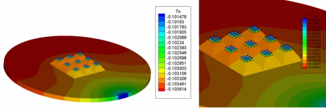
In [65], Huang et al. have applied an adaptive new-version FMM to solve the steady Stokes equations. This algorithm is the basis for the software package FMMStokes. The solver has been applied to the simulation of Stokes flow inside a micro-fluidic device with complex geometry. This device consists of two parallel circular plates, with 81 spouts placed on the top. The bottom plate is moving with axial symmetrical normal velocity. The inlet and spouts are specified by traction boundary conditions; zero-velocity boundary conditions are specified on other surfaces. In the simulation, the device is discretized into 279,046 triangular elements. In the adaptive FMM, 18 trems in the multipole, local and exponential expansions were used. The CPU time requirement for the problem with more than 106 unknowns is about 3 hours, substantially more efficient
than other existing solvers. In Figure 1.1, the contour plot of the surface normal traction is shown, which is good agreement with observed experimental results.
Figure 1.1: Normal stress distribution (left) and its zoomed view (right)
Figure 1.2: Parallel speedup vs. number of processors
ScaLapack based methods. In fact, this is a challenge brought forth by the adaptive FMM.
can compute the electrostatic field of a small-scale molecule system (about 100,000 un-knowns) in less than 10 seconds on today’s desktop and reduce the time for very large molecule structure from days by other software tools to 20 minutes with AFMPB. In has also been tested on different biomolecule systems including the nicotinic acetylcholine receptor (nAChR), and interactions between protein Sso7d and DNA. The software has been released under open source license agreements, and there are already interests in in-corporating this package into other commonly used tools for molecular dynamics simula-tions. AFMPB has made a significant and critical leap, in terms of arithmetic complexity and numerical stability, towards the simulations of electrostatics of large-scale systems in protein-protein interactions and nano particle assembly processes. Its potential is yet to be fully explored on modern and emerging multicore or multi-processors computing sys-tems for simulating a very large molecular system such as in protein-protein interacitons or molecular binding, where millions of such evaluations are required. By estimation, we expect that the time for calculating the electrostatic field to be within one second in order to perform the dynamical simulation within a reasonable time frame. In other words, an order or two of magnitude in speed-up is expected.
In [79], a new-version FMM was applied to calculate the stress field of dislocation ensembles due to the long-range interaction of dislocations that are the primary carriers of plastic deformation in crystals. Their numerical results show that the new algorithm is very efficient and accurate, and can evaluate the stress field of a large number of dislocations. However, the presented algorithm is currently designed only for dislocation ensembles in isotropic media, where the interactions can be modeled by the biharmonic kernels. In order to incorporate the elastic anisotropy, new algorithms are required for the anisotropic Green’s function commonly used in material science studies.
new-version FMM codes for the scientific computing community; (2) their paralleliza-tion on multicore machines using multi-threading techniques; and (3) generalized kernel independent FMM for a wider class of kernels.
Chapter 2
Fast Multipole Method
In the numerical simulation of many physical processes, the rapid evaluation of the pair-wise interactions of N particles is required. Examples include the dynamics of charged particle clusters governed by the Newton’s law of motion in the electrostatic field, and the solution of equations for the gravitational interactions in the study of astrophysics. Given N particles each carrying a charge qi (or mass mi) at location xi = (xi, yi, zi), the electrostatic (or gravitational) potential field is described by
Φ(xj) = N
X
i=1
i6=j
qi kxi−xjk
, (2.1)
and the corresponding force field can be computed by means of F = −∇Φ. In this formula, the Coulomb interaction 1
r is assumed wherer is the distance between two par-ticles. Other interactions include the screened Coulomb potential e
−kr
r (k ∈ R
+), the
Lennard-Jones potential, and the hydrodynamics interactions described by the Oseen tensor. Equation (2.1) also arises in the integral equation methods when a convolu-tion ´ G(x, y)q(y)dy of the Green’s function (kernel) G(x, y) and a given density q(y) is discretized using quadrature rules. Equation (2.1) can be equivalently represented as a matrix-vector multiplication, with the matrix having zeros on the diagonal and
{ 1
kxi−xjk
multipli-cation) in Equation (2.1), O(N2) operations are required, which becomes prohibitive for
large-scale problems even on modern supercomputers. Indeed, the advance in computer architectures requires innovative numerical algorithms. In particular, the asymptotically optimalO(N) methods for the special structured matrix vector operations are in urgent need in science and engineering applications.
There have been numerous research efforts to develop O(N) or O(NlogN) algo-rithms for the summation in Equation (2.1), including the Fast Fourier Transform (FFT) based algorithms (e.g., Particle Mesh (PM) , Particle-Particle Particle-Mesh (P3M) [38], Particle Mesh Ewald (PME) [21], pre-corrected FFT [57]), multi-wavelet based schemes [37], multigrid multi-level methods [15], and the multipole expansion tech-niques [5, 6, 34, 35]. In this thesis, we focus on the multipole expansion techtech-niques first studied by Appel [5] and Barnes and Hut [6]. In their “tree-code” algorithm, the complexity is reduced to O(NlogN) by using a low order spherical harmonics expan-sion to represent the “far-field” of a cluster of particles and a downward (or upward) pass to transmit this “multipole” expansion to the “interaction” list. In 1987, by in-troducing the additional local expansion and using both the upward and downward passes, Greengard and Rokhlin invented the asymptotically optimal O(N) fast multi-pole method (FMM) and applied it to many-body problems [34]. The FMM was elected as one of the top ten algorithms for the twentieth century and it has been successfully applied in many science and engineering fields such as computational electromagnetic [59, 60, 32, 18, 48, 49, 81, 82], molecular dynamics [14, 31, 45, 47, 40], computational fluid and solide mechanics [33, 26, 63, 69, 73, 72, 74], etc.
efficiency, Greengard and Rokhlin published a new-version FMM [35] for the Coulomb potential after ten years of hard work. In the new-version FMM, an intermediate “plane-wave” representation is introduced to diagonalize the most expensive “multipole-to-local” translation operator, and a “merge-and-shift” technique is applied to reduce the number of such translations. As a result, the new-version FMM can be orders of magnitude faster compared with its original version, especially in 3D. Specifically, the 3D new-version FMM breaks even with direct interaction (estimation of the prefactor in O(N)) at approximatelyN = 750 for three digits accuracy andN = 1500 for six digits accuracy, compared with tens of thousands for the original version. The details of the original and new version of FMM will be discussed in subsequent sections, and we refer interested readers to [39] for the new version of FMM for the Laplace equation in 2D, to [71] for an improved technique in 1D, to [24] for a new-version FMM accelerated Poisson solver in 2D, and to [20] for the adaptive implementation details for the Laplace equation in 3D.
The new-version FMM has also been generalized to other kernels, including the screened Coulomb potential, the Helmholtz Green’s function, and the biharmonic kernel. In particular, in [32], a new-version FMM was developed for the low-frequency Helmholtz equation in 3D by separating the Helmholtz Green’s function into the evanescent and propagating parts and introducing the exponential expansions. This technique was later combined with a high-frequency FMM code based on a different diagonal translation operator as described in [60], resulting in the so-called “wideband” FMM [18]. We want to mention that the diagonal technique in the low-frequency regime is very different from that in the high-frequency regime: the complexity of the low-frequency diagonal scheme is O(N2) when used in the high-frequency regime while the diagonal scheme for
for the Maxwell equations in [52], the elastic wave propagations [76, 77, 78], and the more recent fast direct solvers using the low separation rank properties in the FMM algorithms [19, 50].
The new-version FMMs for the commonly used Coulomb, screened Coulomb, and Helmholtz kernels are considered well-studied subjects. In this chapter, we focus on the screened Coulomb interaction Φ = e
−λr
2.1
Spatial Domain Adaptive Tree Structure
Unlike the algebraic structure based FFT algorithm, the FMM algorithm uses a data structure based on the spatial domain adaptive oct-tree for data communication. In this section, we describe how to construct the adaptive oct-tree and the corresponding data structure. Interested readers are also referred to [20] where the adaptive tree and data structure are discussed for the new-version FMM for the Laplace equation (Coulomb potential).
Given N particles, the new-version FMM starts with constructing an adaptive oct-tree consisting of a hierarchy of boxes. The root box, which is referred to as refinement level 0, is the smallest Cartesian box containing allN particles. Starting from level 0, we recursively obtain levell+ 1 through subdivision of the boxes at levell with more thans particles into eight boxes of equal size, where s is some pre-specified integer parameter. At each level of refinement, a table of non-empty boxes is maintained, so that once an empty box is encountered, its existence is forgotten and it is completely ignored by the subsequent process.
In this structure, a box is called a parent box if it contains more than s particles. Otherwise, it is referred to as a childless box or leaf box. A box cis said to be thechild of box b if box c is obtained by a single subdivision of box b. On the other hand, such a box b is the parent of box c. Boxes resulting from the subdivision of a parent box are referred to as siblings. Thecolleagues of a boxb consist of the boxes at the same level of b sharing at least one point with b, including box b itself. Apparently, a given box can have up to 27 colleagues in three dimensions.
One key observation in the FMM algorithm is the so-called “low separation rank” property for the well-separated boxes in the oct-tree structure. We say two sets{xi}and {yi} are well-separated if there exists points x0 and y0 ∈ R3 and a real number r > 0
|xi−x0|< r ∀i= 1, . . . , m
|yj −y0|< r ∀j = 1, . . . , n, and
|x0−y0|> c·r, (2.2)
where c is bounded below by some constant c0 > 2. Two boxes B1 and B2 of the
same size in the oct-tree structure are said to be well-separated if they are at least one box of the same size apart, i.e., if any sets of points {xi} ⊂ B1 and {yi} ⊂ B2 are
well-separated (with c0 =
4 √
3). As will be discussed in the next section, “information” in two well-separated boxes can be compressed either analytically using special basis functions (e.g., spherical harmonics for Laplace kernels) or numerically using singular value decomposition (SVD) before being sent out.
Well-separated boxes can also appear at different levels in the oct-tree structure. Assume that a box b can inherit information from its parentcwhile traversing down the tree structure, which contains the information from all well-separated boxes of c. Then we can define the interaction list of b as the union of boxes at the same level of b that are well-separated from b, but whose parents are not well-separated from b’s parent c. Clearly, the information received from b’s parent and the interaction list is equivalent to the information from all well-separated boxes of b.
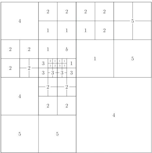
For a given box b in the adaptive oct-tree structure, it may also need to “communi-cate” with boxes of different sizes. In Figure 2.1, we associate b with five lists of other boxes, determined by their positions with respect to b. We store list and pointers for parent-child relations for each box in the oct-tree structure.
In the following, we give the detailed definition for each list.
b
1
1 1 1
1
1
1 1 1
2 2 2 2
2
2 2
2 2
2 2
2 2
3
3 3 3 3
3 3 3 3 3
4 4
4
5
5 5
5
• List 2 of a box b will be denoted by Vb and is formed by all the children of the colleagues of b’s parent that are well separated from b. List 2 is also referred to as the interaction list.
• List 3 of a box b will be denoted by Wb. Wb is empty if b is a parent box, and consists of all descendants of b’s colleagues whose parents are adjacent to b, but who are not adjacent to b themselves, if b is a childless box. Note b is separated from each boxw inWb by a distance greater than or equal to the length of the side of w.
• List 4 of a box b will be denoted by Xb and is formed by all boxes c such that b∈Wc. Note that all boxes in List 4 are childless and larger than b.
• List 5 of a box b will be denoted by Yb and consists of all boxes that are well separated fromb’s parent.
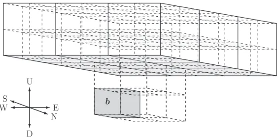
In the new-version FMM, plane-wave expansions are introduced to diagonalize the multipole-to-local translation from box b to its interaction list boxes to reduce the huge prefactor inO(N). As the plane-wave expansions have directions, each boxbis associated with six such expansions, each emanating from one face of the cube. Consequently, the interaction list for each box is further subdivided into six lists, associated with the six coordinate directions (+z,−z, +y,−y, +x,−x) in the three dimensional coordinate sys-tem. We will refer to the +z-direction as up, the −z-direction as down, the +y-direction as north, the −y-direction as south, the +x-direction as east, and the −x direction as west.
The Uplist is demonstrated in Figure 2.2, and the definition for each list is given below:
b
U
D
W E
S
N
Figure 2.2: The U plistfor the box (b)
2. The Downlist for a box b consists of those elements of the interaction list which lie below b and are separated by at least one box in the −z direction.
3. The Northlist for a box b consists of those elements of the interaction list which lie north of b, are separated by at least one box in the +y-direction, and are not contained in the Up or Down lists.
4. The Southlist for a box b consists of those elements of the interaction list which lie south of b, are separated by at least one box in the −y-direction, and are not contained in the Up or Down lists.
5. The Eastlist for a box b consists of those elements of the interaction list which lie east of b, are separated by at least one box in the +x-direction, and are not contained in the Up, Down, North, or South lists.
6. The Westlist for a box b consists of those elements of the interaction list which lie west of b, are separated by at least one box in the −x-direction, and are not contained in the Up, Down, North, or South lists.
[54], White et al. described another variant of the oct-tree and data structure used in FMM. In their scheme, a neighbor of a given cube is defined as any cube which shares a corner with the given cube (nearest neighbor) or shares a corner with the nearest neighbor (second-nearest neighbor). The interaction list of a cube is the set of cubes that are either the second-nearest neighbors of a given cube’s parent or are children of the given cube’s parent’s nearest neighbors excluding the nearest or second-nearest neighbors of the given cube. The advantage of this approach is that fewer terms can be used in the multipole and local expansion since the “ interacting” boxes are further apart. However, this will significantly change the implementation and performance of the plane-wave expansions in the new-version FMM. It is unclear which data structure is superior. As will be discussed in the next chapter, one of my future research projects is to generate a graph with nodes representing different interactions of the boxes and edges the associated costs, and study the “optimal” connecting tree on parallel computer architectures.
2.2
Approximations and Translations
Another important concept in the FMM algorithm is the extraction, storage, and trans-mission of the data (or “information”) based on the oct-tree structure. In this section, using Yukawa potential as an example, we introduce the analytical spherical harmon-ics expansions and the plane-wave approximation, and discuss the translation operators which transmit the “information” from one box to another. Specifically, givenN charges q1, q2, . . . , qN at the locationx1,x2, . . . ,xN in R3, we consider the pairwise interactions
Φ(xj) =
N
X
i=1
i6=j qi·
e−λkxj−xik
kxj−xik
, λ ∈ R+, (2.3)
neglect their proofs in this section, and refer interested readers to [31] for further details. First, we study how to collect and compress the “information” from particles inside a box c using the multipole expansion as described in the following theorem.
Theorem 2.1 (Multipole Expansion (TSM operator)). Suppose that box c centered at the origin contains N sources of strengths q1, q2, . . . , qN located at points x1,x2, . . . ,xN with spherical coordinates (ρ1, α1, β1),(ρ2, α2, β2), . . . ,(ρN, αN, βN), respectively. Then the potential for any point x= (r, θ, φ) outside box c is given by a multipole expansion
Φ(x) = N
X
i=1
qi·
e−λkx−xik
kx−xik = 2λ
π N
X
i=1
qi·k0(λkx−xik)
= ∞ X n=0 n X
m=−n
Mnmkn(λr)·Ynm(θ, φ), (2.4)
where the multipole coefficients are
Mnm = 8λ N
X
i=1
qi·in(λρi)·Yn−m(αi, βi). (2.5)
Furthermore,
Φ(x)− p
X
n=0
n
X
m=−n
Mnmkn(λr)·Ynm(θ, φ)
=Oa r
p
, (2.6)
where a is the radius of the smallest sphere enclosing box c.
In the formulas, Ym
n is the spherical harmonics of degreen and order m defined by
Ynm(θ, φ) =
r
2n+ 1 4π
s
(n− |m|)! (n+|m|)!·P
|m|
n (cosθ)e imφ
, (2.7)
where the associated Legendre functions Pm
poly-nomial Pn(x) by Rodrigues’ formula
Pnm(x) = (−1)m(1−x2)m/2 d
m
dxmPn(x), (2.8)
and the modified spherical Bessel and modified spherical Hankel functions in(r), kn(r) are defined in terms of the usual Bessel function Jν(z) via
Iν(r) =i−νJν(ir) (i= √
−1), Kν(r) = π
2 sinνπ[I−ν(r)−Iν(r)] in(r) =
r
π
2rIn+1/2(r), kn(r) =
r
π
2rKn+1/2(r).
Notice that we have a
r < 1 when two boxes are well-separated, hence the expansion decays rapidly as p increases.
Next, we describe how to store the collected far-field “source” particle information in a local expansion, which is valid for all the “target” particles in the box which is well-separated from the box containing the source particles.
Theorem 2.2 (Local Expansion (TSL operator)). Suppose that N sources of strengths q1, q2, . . . , qN are located at the points x1,x2, . . . ,xN in R3 with spherical coordinates (ρ1, α1, β1), (ρ2, α2, β2), . . . ,(ρN, αN, βN), respectively. Suppose further that all the points
x1, x2, . . . ,xN are located outside the sphere Sa of radius a centered at the origin. Then, for any pointx∈Sawith coordinates(r, θ, φ), the potentialΦ(x)generated by the sources q1, q2, . . . , qM is described by the local expansion
Φ(x) =
∞
X
j=0
j
X
k=−j
Lkjij(λr)·Yjk(θ, φ), (2.9)
where
Lkj = 8λ N
X
l=1
Furthermore,
Φ(x)− p
X
j=0
j
X
k=−j
Lkjij(λr)·Yjk(θ, φ)
=O r a p . (2.11)
In the tree-code algorithm, for each box at a certain level in the tree structure, its multipole expansion is formed by collecting information from the particles inside the box. As a result, at least O(N) operations are required for each level to account for communication with N particles. Notice that the tree has approximately logN levels, hence the complexity of tree-code algorithm is at least O(NlogN). In order to reduce the cost in forming multipole expansions for all boxes, in the original FMM [34], a divide-and-conquer strategy is applied. For each parent box, instead of communicating with the particles directly, its multipole expansion is derived by shifting and merging its chil-dren’s multipole expansions (which already contain the collected and compressed particle information) using the following multipole-to-multipole (TM M) translation operator: Theorem 2.3 (TM M translation). Consider a box b centered at the origin and its child c centered at x0 = (ρ, α, β), and a point x= (r, θ, φ) in the far-field boxes of b. Assume
the potential due to charges in box c is given by the multipole expansion
Φ(x) =
∞
X
n=0
n
X
m=−n
Omnkn(λr0)·Ynm(θ
0
, φ0), (2.12)
where (r0, θ0, φ0) are the spherical coordinates of the vector x−x0. Then, the field can
also be described by a shifted multipole expansion:
Φ(x) =
∞
X
n=0
n
X
m=−n
Mnmkn(λr)·Ynm(θ, φ). (2.13)
The linear operator mapping the old multipole coefficients {Omn} to the new multipole coefficients {Mnm} is denoted by TM M.
from refinement level 0 to the finest level is performed to form each box’s local expansion which contains the far-field particle contributions. For a box cat level l, a translation is first carried out to shift its parentb’s local expansion (which contains particle information fromb’s far-field) to an equivalent local expansion about the center of boxc, via the local-to-local (TLL) operator as follows:
Theorem 2.4 (TLL translation). Consider a point x = (r, θ, φ) in box c and the local expansion of c’s parent box b
Φ(x) = p
X
n=0
n
X
m=−n
Lmnin(λr)·Ynm(θ, φ). (2.14)
Assume box c is centered at x0 = (ρ, α, β), then the local expansion of c is given by
Φ(x) = p
X
n=0
n
X
m=−n
Nnmin(λr0)·Ynm(θ
0
, φ0), (2.15)
where (r0, θ0, φ0) are the spherical coordinates of the vector x−x0. The linear operator
mapping the old local coefficients {Lm
n} to the new local coefficients {Nnm} is denoted by TLL.
In the second step of the downward pass, box creceives contributions from particles which are located inside a region formed by subtracting its parentb’s far-field from its own far-field. Boxes in this region are members of the aforementioned list 2 or the interaction list of the given boxc. Instead of communicating with the particles in this region directly, a multipole-to-local translation (TM L) is performed to convert the multipole expansions of each interaction list box into a local expansion which is then merged into c’s local expansion. TheTM L translation operator is defined as follows:
Theorem 2.5 (TM L translation). Suppose box b centered at x0 = (ρ, α, β) is an
to charges in b can be described by a local expansion
Φ(x) =
∞
X
j=0
j
X
k=−j
Lkjij(λr)·Yjk(θ, φ). (2.16)
The linear operator mapping the multipole coefficients {Mm
n } to the local coefficients {Lm
n} is denoted by TM L.
At the end of the downward sweep, we evaluate local expansion at every particle location in each childless box, and then compute the near-field interactions directly.
Recall that in three dimensions, the interaction list of a given box can contain up to 189 boxes. Additionally, the operation complexity of theTM Loperator isO(p4) assuming p2 terms are used in each expansion. Consequently, this original multipole-to-local
trans-lation requires prohibitive 189p4 operations for each box, which makes the original FMM
less attractive to large-scale problems. Therefore, we next introduce the plane-wave ex-pansions analogous to the work of Greengard and Rokhlin in [35] to diagonalize theTM L operator. In three dimensions, six different plane-wave expansions are introduced for each face of the box. We use the upward (or +z) direction to illustrate the idea and omit the details of other directions which can be processed in a similar manner. For boxes in the uplist of a box (see Figure 2.2), its multipole expansion is first translated into an exponential expansion by the multipole-to-exponential (TM E) operator as follows:
Theorem 2.6 (TM E translation). For a point x in the up direction with spherical co-ordinates (r, θ, φ), assume the potential φ(x) is approximated by the truncated multipole expansion (due to charges in box c centered at the origin) with error bound
Φ(x)− p
X
n=0
n
X
m=−n
Omn ·Ynm(θ, φ)kn(λr)
then with error bound O(), Φ(x) can be approximated by
λ s() X
k=1
Mk X
j=1
W(k, j)·e−(uk+λ)z·ei
√
uk+2ukλ·(xcosαj,k+ysinαj,k), (2.18)
where (x, y, z) are the Cartesian coordinates of x, the coefficients W(k, j) are given by
πwk 2λMk
p
X
m=−p
i|m|eimαj,k
p
X
n=|m|
Omn
r
2n+ 1 4π
s
(n− |m|)! (n+|m|)!P
|m|
n
λ+uk λ
, (2.19)
for k = 1, . . . , s(), j = 1, . . . , Mk. The linear mapping from {Onm} to {W(k, j)} is referred to as the TM E translation operator.
In Equation (2.18), the weights wk and nodes uk are computed according to the generalized Gaussian quadrature as discussed in [70]. Once the multipole expansion is converted into the exponential expansion about the center of box c (the origin), shifting it to a new centerx0 = (x0, y0, z0) of an interaction list box of ccan be done diagonally,
as described by the exponential-to-exponential (TEE) operator as follows:
Theorem 2.7 (TEE translation). For the exponential expansion in Equation (2.18) of box c centered at the origin and a box in the interaction list centered at x0 = (x0, y0, z0),
the shifted exponential expansion for any point (x, y, z) is given by
s() X
k=1
Mk X
j=1
V(k, j)·e−(uk+λ)(z−z0)ei √
u2
k+2ukλ·((x−x0) cosαj,k+(y−y0) sinαj,k), (2.20)
where
V(k, j) =W(k, j)·e−(uk+λ)z0 ·ei √
u2
k+2ukλ·(x0cosαj,k+y0sinαj,k), (2.21)
fork = 1, . . . , s(),j = 1, . . . , Mk. The linear operator mapping the coefficients{W(k, j)} to the coefficients {V(k, j)} is denoted byTEE.
the exponential expansions can be translated to a local expansion about the box center using the exponential-to-local (TEL) operator as follows:
Theorem 2.8 (TEL translation). Suppose that the potential for x= (x, y, z) is given by Equation (2.18), then there exists an integer p, such that
Φ(x)− p
X
n=0
n
X
m=−n
Lmnin(λr)Ynm(θ, φ)
=O(), (2.22)
where (r, θ, φ) are the spherical coordinates of x with respect to the box center and
Lmn = (−1)ni|m|√
4π√2n+ 1
s
(n− |m|)! (n+|m|)!
s() X
k=1
Pn|m|
uk+λ λ
Mk X
j=1
W(k, j)eimαj,k (2.23)
forn = 0, . . . , p,m =−n, . . . , n. The linear operator converting the coefficients{W(k, j)} into the coefficients {Lm
n} is denoted by TEL.
From the complexity perspective, by using the decompositionTM L=TEL◦TEE◦TM E, the previous prohibitive 189p4 operation counts are now reduced to approximately 2p4+
189p2, which potentially can be further reduced to roughly 6p3+ 40p2. To achieve that,
we shall first apply the point-and-shoot technique and rotate the multipole expansion so that TM E operator can be performed along the z-axis (3p3 operations, more details in [35]). Next, the exponential expansions of box cand its siblings shall be merged before being sent out to their common interaction list boxes, which reduces the operations from 189p2 to 40p2. Lastly, we shall translate each box’s exponential expansion into a local
2.3
Algorithm Structure of Adaptive FMM
In this section, we present a pseudo-code to explain the algorithmic structure of the adaptive new-version FMM. To simplify our discussions, we introduce the following no-tations. The computational domain is denoted by B0 and the set of all nonempty boxes
at refinement levell is denoted byBl. For each boxb, its associated five lists are denoted by Ub, Vb, Wb, Xb, Yb, respectively. Vb is further subdivided into U plist(b), Downlist(b), N orthlist(b),Southlist(b),Eastlist(b), andW estlist(b) to utilize the plane-wave expan-sions. Also, each box b is associated with the following fourteen expansions:
• A multipole expansion Φb of the form (2.4) representing the potential generated by charges inside b; it is valid in R3\ {U
b∪Wb}.
• A local expansion Ψb of the form (2.9) representing the potential generated by all charges outside Ub ∪Wb; it is valid inside box b.
• Six outgoing exponential expansions WbU p, WDown
b , WbN orth, WbSouth, WbEast, and WW est
b of the form (2.18), representing the potential generated by all charges located inside b and valid in U plist(b), Downlist(b), N orthlist(b), Southlist(b), Eastlist(b), and W estlist(b), respectively.
• Six incoming exponential expansionsVbU p,VbDown,VbN orth,VbSouth,VbEast, andVbW est of the form (2.18), representing the potential inside b generated by all charges in Downlist(b), U plist(b), Southlist(b), N orthlist(b), W estlist(b), and Eastlist(b), respectively.
Pseudo-Code: Adaptive FMM Algorithm
Initialization
Generating Oct-Tree Structure
Step 1
for l = 0,1,2, . . .
for each box b∈Bl
if b contains more than s particles then
Divide b into eight child boxes. Ignore empty children and add the nonempty child boxes to Bl+1.
endif
end
end
Comment[Denote the maximum refinement level obtained bylmaxand the total number of boxes created by nboxes.]
for each box bi, i= 1,2, . . . , nboxes Create Lists Ubi, Vbi, Wbi, Xbi.
Split Vbi into U p, Down, N orth, South, East, W estlists.
end
Upward Pass
Step 2
for l =lmax, . . . ,−1,0 for each box b inBl
if b is childless then
Use operator TM M to merge multipole expansions from its children into Φb. endif
end
end
Downward Pass
Step 3
Comment [For each box b, add to its local expansion the contribution due to particles inXb. ]
for each box bi, i= 1, . . . , nboxes for each box c∈Xbi
if the number of particlesbi ≤p2 then
Comment [The number of particles in bi is small. It is faster to use direct calculation than to generate the contribution to the local expansion Ψbi
due to charges in c; act accordingly.]
Calculate potential field at each particle point in bi directly from particles in c.
else
Comment [The number of particles in bi is large. It is faster to generate the contribution to the local expansion Ψbi due to particles inc than to
use direct calculation; act accordingly.]
Generate a local expansion at bi’s center due to particles in cusing Theorem 2.2, and add to Ψbi
endif
end
Step 4
Comment [For each box b on level l with l = 2,3, . . . , lmax and each direction Dir = U p, Down, N orth, South, East, W est, create from box b’s multipole expansion the out-going exponential WDir
b in direction Dir, using Theorem 2.6. Translate WbDir to the center of each box c∈Dirlist(b) using Theorem 2.7 and add the translated expansions to its incoming exponential expansion VcDir. Lastly, convert VcDir into a local expansion using Theorem 2.8 and add it to Ψc.]
for l = 2,3, . . . , lmax
for Dir =U p, Down, N orth, South, East, W est for each box b∈Bl
Convert Φb into WbDir by Theorem 2.6. for each box c∈Dirlist(b)
TranslateWbDir to the center of box cusing Theorem 2.7. Add the translated expansion toVcDir.
end
end
for each box c∈Bl Convert VDir
c into a local expansion using Theorem 2.8, and add it to Ψc.
end
end
end
Step 5
Comment[For each parent boxb, shift the center of its local expansion to its children.]
if bi is a parent box then
Shift the local expansion Ψbi to the centers of its children using the operator
TLL, and add the translated expansions to children’s local expansions. endif
end
Evaluation of Potentials
Step 6
Comment [Evaluate the local expansion at leaf nodes.]
for each box bi = 1,2, . . . , nboxes if bi is childless then
Calculate the potential at each charge in bi from the local expansion Ψbi.
endif
end
Step 7
Comment [For each childless boxb, evaluate the potential due to particles in Wb. ]
for each box bi, i= 1,2, . . . , nboxes if bi is childless then
for each box c∈Wbi
if the number of charges in c≤p2 then
Comment[The number of charges in cis small. It is faster to use direct calculation than to evaluate the multipole expansion Φc.] Calculate the potential at each chargebi directly from
else
Comment[The number of charges in cis large. It is faster to evaluate the expansion Φc than to use direct calculation.] Calculate the potential at each charge in bi
from multipole expansion Φc endif
end
endif
end
Step 8
Comment [Local direct interactions.]
for each box bi, i= 1,2, . . . , nboxes if bi is childless then
Calculate the potential at each charge in bi directly due to all charges in Ubi
endif
end
2.4
FMM-Yukawa in FMMsuite
under GPL 2.0 license agreement. The website also hosts many educational and research resources on integral equation methods and fast algorithms.
Figure 2.3: Screenshot of Fast Multipole Methods website
In this section, we present the details of the FMM-Yukawa solver in the FMMSuite package, including the installation instructions, a sample driver file, and several numerical experiments to demonstrate the performance of the solver. The manual for the FMM-Yukawa solver can also be found in [40].
2.4.1
FMM-Yukawa Installation Instructions
After the package is downloaded and extracted to local computer, the user will find the following directories:
• doc: contains license and readme.txt
• src: source files and makefile
The package has been successfully complied using the IntelR complier for Linux and
The main driver for FMM-Yukawa is called “adapyukdriver.f”. The main function is FMMYUK-A in the file “fmmadapyuk.f”, which calls the subroutine D3MSTRCR to generate the adaptive tree structure, and YADAPFMM for calculating the force field and potential. There are three important parameters defined in the header file “parm-ayuk.h”. NBOX is the maximum number of particles (s) allowed in a childless box; NTERMS is the number of terms in first summation of the multipole and local ex-pansions; NLAMBS is the number of terms in the first summation of the exponential expansion. Currently only three- and six- digits accuracies are allowed, and more options will be added in future updates. Input variables include the screening factor BETA, the number of charges NATOMS, charge locations ZAT(3,NATOMS), and the charge CHARGE(NATOMS) carried by each particle. FMM-YUKAWA will calculate and out-put the potential POT(NATOMS) and the field FIELD(3,NATOMS).
2.4.2
A Sample Driver File
In this section, we provide a sample driver file to explain how FMM-YUKAWA can interact with other existing codes.
A driver file for FMM-Yukawa
IMPLICIT NONE
INTEGER *4 NATOMS,IER
PARAMETER (NATOMS=1000000)
REAL *8 BETA
REAL *8 ZAT(3,NATOMS),CHARGE(NATOMS)
REAL *8 POT(NATOMS),FIELD(3,NATOMS)
c
c—set up parameters.
BETA=0.1D0
c
c—generate charges and their locations.
c
CALL DUMMY(NATOMS,ZAT,CHARGE)
c
c—call fmm to calculate the potential and field.
c
CALL FMMYUK A(BETA,NATOMS,ZAT,CHARGE,POT,FIELD,IER)
c
STOP
END
2.4.3
Test Run Description
In this section, we present two numerical examples to show the efficiency and accuracy of the
FMM-Yukawa package. In the experiment, we use a machine with IntelR T9400 processor at
2.53 GHz clock rate and 3GB memory. The results are summarized in Tables 2.1 – 2.4. In
the table, N is the number of particles for which calculations have been preformed; s is the
maximum number of particles allowed for a childless box (for each N, we run the program
with multiple choices of s and the one yielding the optimal timing is reported here); lmax is the maximum number of refinement of the tree structure;nboxes is the total number of boxes
created; Tf mm and Tdir refer to the timing results for FMM algorithm and direct calculation, respectively. In the table, all timings are given in seconds and the storage is measured in
megabytes.
In the tests, we consider two distributions of the particles, namely, uniformly distributed
inside a unit box [−0.5,0.5]3 and on a spherical surface centered at the origin of radius 0.5.
For each distribution, we run the program with three- and six- digit accuracy. The screening
and the actual FMM calculation time. Tdir is estimated by extrapolating the CPU time for evaluating the potentials at 400 particle locations directly since calculating the entire system
in this fashion would require prohibitive amounts of CPU time without providing much useful
information. Similarly, the accuracy of the algorithm is calculated at those locations according
to the formula
E = v u u u u u u u u t 400 X i=1
Φ(xi)−Φ(˜ xi) 2 400 X i=1
|Φ(xi)|2
, (2.24)
where Φ(xi) is the result obtained from direct calculation and ˜Φ(xi) is the result obtained from FMM algorithm.
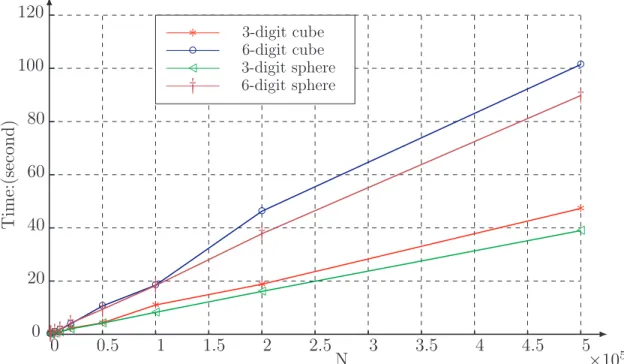
For each table, the timing results are further plotted as a function of N (see Figure 2.4).
In the figure, we can observe that the actual CPU time required by the FMM-Yukawa package
grows approximately linearly with N. Lastly, we want to mention that the numerical results
suggest that the break-even point of the new version FMM is roughly 750 for three-digit and
1500 for six-digit accuracy, which is an estimate of the constant associated with O(N) in the
complexity analysis.
N s lmax nboxes p Sexp Storage Tf mm Tdir Error
750 40 2 41 9 67 1.20 0.07 0.08 9.7·10−5
1500 30 3 165 9 67 1.90 0.15 0.32 1.7·10−4
5000 30 4 649 9 67 4.60 0.40 3.4 1.9·10−4
10000 40 4 681 9 67 5.08 0.77 14 2.6·10−4
20000 30 5 4729 9 67 26.44 2.25 54 3.6·10−4
50000 30 5 4776 9 67 28.52 4.29 337 3.5·10−4
100000 40 5 4777 9 67 31.57 11.02 1349 4.4·10−4
200000 40 6 33506 9 67 184.97 18.82 5480 4.6·10−4
500000 40 6 37363 9 67 223.05 47.32 33900 4.6·10−4
N s lmax nboxes p Sexp Storage Tf mm Tdir Error
750 70 2 41 18 311 3.05 0.16 0.08 5.9·10−8
1500 50 3 81 18 311 3.92 0.32 0.32 6.8·10−8
5000 50 4 197 18 311 6.52 0.91 3.4 1.1·10−7
10000 50 4 681 18 311 16.76 1.71 14 1.5·10−7
20000 80 4 681 18 311 17.37 3.86 54 1.8·10−7
50000 80 5 4776 18 311 103.31 10.65 337 2.3·10−7
100000 80 5 4777 18 311 106.38 18.47 1349 2.8·10−7
200000 80 6 4945 18 311 115.94 46.27 5480 2.5·10−7
500000 60 6 37363 18 311 800.06 101.45 33862 3.9·10−7
Table 2.2: Timing results for FMM-Yukawa for 6-digit accuracy with charges uniformly distributed inside the cube [−0.5,0.5]3
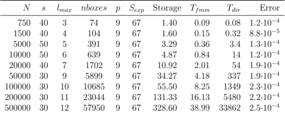
N s lmax nboxes p Sexp Storage Tf mm Tdir Error
750 40 3 74 9 67 1.40 0.09 0.08 1.2·10−4
1500 40 4 104 9 67 1.60 0.15 0.32 8.8·10−5
5000 50 5 391 9 67 3.29 0.36 3.4 1.3·10−4
10000 50 6 639 9 67 4.87 0.84 14 1.2·10−4
20000 40 7 1702 9 67 10.92 2.01 54 1.9·10−4
50000 30 9 5899 9 67 34.27 4.18 337 1.9·10−4
100000 30 10 10685 9 67 55.50 8.25 1349 2.3·10−4
200000 30 11 23044 9 67 131.33 16.13 5480 2.2·10−4
500000 30 12 57950 9 67 328.60 38.99 33862 2.5·10−4
Table 2.3: Timing results for FMM-Yukawa for 3-digit accuracy with charges distributed on the surface of a sphere
N s lmax nboxes p Sexp Storage Tf mm Tdir Error
750 70 2 65 18 311 3.55 0.17 0.08 1.0·10−7
1500 60 3 100 18 311 4.31 0.31 0.32 7.1·10−8
5000 60 5 323 18 311 9.11 0.93 3.4 0.5·10−8
10000 50 6 639 18 311 15.90 1.79 14 8.7·10−8
20000 40 7 1702 18 311 38.34 4.17 54 1.0·10−7
50000 80 7 2079 18 311 47.92 9.39 337 1.6·10−7
100000 60 9 5976 18 311 131.01 18.32 1349 1.8·10−7
200000 60 10 10987 18 311 240.03 37.81 5480 1.7·10−7
500000 50 12 32715 18 311 704.60 89.79 33862 1.8·10−7
∗ 3-digit cube
◦ 6-digit cube
/ 3-digit sphere
† 6-digit sphere
0 0.5 1 1.5 2 2.5 3 3.5 4 4.5 5
×105
0 20 40 60 80 100 120
Time:(second)
N
∗∗∗∗∗ ∗
∗
∗
∗
◦◦◦◦◦ ◦
◦
◦
◦
//// / /
/
/
/
††††† †
†
†
†
Chapter 3
Parallelization of Fast Multipole
Method on Multicore Architectures
In this chapter, we focus on the parallelization of FMM to further accelerate the performance
of the algorithm. Particularly, we will discuss available options in architecture platforms and
develop parallelization strategies. It is well known that parallelization is one of the crucial
fac-tors left for further acceleration of the FMM algorithm since the complexity of the sequential
FMM has already been pushed to its own limit with the introduction of plane-wave expansion.
Although the new-version FMM breaks even with direct calculation at N = 750 for 3-digit
accuracy and N = 1500 for 6-digit accuracy, which is a remarkable accomplishment, it still
consumes prohibitively large amount of time in many large-scale simulations (hundreds of
mil-lions unknowns) of biomolecular, physical and chemical systems. There is an urgent need to
further accelerate FMM algorithm by another two or three orders to enable those important
research at affordable costs. Therefore, we propose a parallel new-version adaptive FMM based
on graph-theoretic approach in this chapter.
This chapter is organized as follows. In Section 3.1, we provide a brief overview of the
development of FMM in the last two decades, in terms of the algorithm employed, particle
distribution, architecture topology, and the application contexts. In Section 3.2, we discuss
the absolute critical path, maximum concurrency potential of the algorithm, and the impact
of architecture constraints on the parallelization. In Section 3.3, we develop a parallelization
strategy following a graph-theoretic approach based on the spatio-temporal partition of the
and report several numerical results to demonstrate the efficiency of the scheme.
3.1
Precursors of Parallel FMM
In this section, we give a brief overview of previous studies and efforts in developing
paral-lel FMM. They differ in terms of the algorithm employed, particle distribution, architecture
topology, and the application contexts.
The parallelization on FMM starts with the uniform version first. The first study comes
from Greengard and Gropp in 1990 on 2D FMM [30]. They showed that withO(N) processors,
the overall complexity isO(logN). They also presented numerical results on a shared memory
machine, the Encore Multimax 320. In 1991, Zhao and Johnsson developed a parallel version
of the 3D uniform FMM using high performance Fortran for the Connection Machine system
model CM-2 [80]. In [41], Board et al. implemented a parallel version of 3D FMM on a
network of workstations using the coordination language Linda [17] and incorporated it into
the molecular dynamics program MD of Windemuth and Schulten [68]. On this distributed
memory system, the authors employed a master-worker scheme. A master process running on
one processor separates the computational work into tasks and sends out one task per processor
to the network. The remaining tasks are then assigned to the processors as they finish their
previously assigned tasks.
Historically, the first successful parallel hierarchicalN-body method for non-uniform particle
distribution on distributed memory systems was obtained by Warren and Salmon [66]. The key
ideas in this paper were the orthogonal recursive bisection (ORB) and locally essential tree
(LET). The idea in ORB partitioning is to recursively divide the computational domain space
into two subspaces with equal costs, until there is one subspace per processor. To provide load
balancing, the cost of a subspace is defined as the sum of the profiled costs of all particles in
the subspace. The idea in LET stems from the following observation. Every body sees only a
fraction of the complete tree. The distant parts are seen at a coarser level of detail while the
nearby sections are seen all the way down to the leaves. As nearby bodies see similar trees, a LET
data that will be required to carry on the computation in the domain. Once the LET is obtained
in an ORB domain, one can proceed exactly as in the sequential case, allowing employing highly
tuned sequential assembly language without regard to communication, synchronization or other
parallel issues. However, ORB and LET introduce several new data structures, including a
binary ORB tree that is distinct from the FMM tree. Additionally, ORB and LET are nontrivial
to implement and debug, and have significant runtime overhead particularly as the number of
processors increases [61]. As a result, other domain decomposition methods based on hashed
tree and space-filling curves have been introduced to achieve better efficiency on the distributed
memory systems.
The hashed oct-tree structure along with space-filling curves was first introduced by Warren
and Salmon [67]. In this paper, instead of using pointers, the topology of the tree is implicitly
represented by mapping the cell spatial locations and levels into keys, which are then translated
into memory locations via a hash table. This scheme provides a uniform addressing mechanism
to retrieve data across multiple processors. It also produces a good domain decomposition by
cutting the one dimensional list of sorted body key ordinates into Np (number of processors) equal pieces, weighted by the amount of work corresponding to each body. Two particular
mappings were studied in the paper, namely, Morton ordering and Peano-Hilbert ordering.
Although the latter provides a better decomposition theoretically, it does not lead to improved
performance in practice.
In [61], the costzone decomposition has been shown to be more efficient than ORB on
common address space architecture. In costzones, the tree is conceptually laid out in a
two-dimensional plane, with a cell’s children laid out from left to right in increasing order of child
number. The cost of every particle is stored with the particle. Every internal cell holds the
sum of the costs of all particles that are contained within it. These cell costs are computed
during the upward pass. The total cost in the domain is divided among processors so that
every processor has a contiguous, equal zone of costs. Which cost zone a particle belongs to is
conceptually determined by the total cost up to that particle in an inorder traversal of the tree.
In the costzones algorithm, processors descend the tree in parallel, picking up the particles
corresponds to contiguity in space, an ordering strategy has been developed. In this solution,
the order in which children are numbered is not the same for all cells. The orderings of a cell
C’s children are determined by: (a) the ordering of C’s siblings; and (b) which child of its
parentC is in that ordering.
A single board of GPUs (graphics processing unit) can be viewed as shared memory at
the API level. The model for GPU computing is to use CPU and GPU together in a
hetero-geneous computing model. The sequential part of the application runs on the CPU and the
computationally-intensive part runs on the GPU. In 2007, Nyland et al. provided an CUDA
(computed unified device architecture) implementation on GPUs computing the pairwise
inter-actions of N bodies using direct interaction method [56]. In 2008, Gumerov and Duraiswami
[36] mapped the original FMM for Laplace kernel onto the GPU architectures. In the current
state, due to bandwidth concerns, the problem size to be handled is approximately in the order
of 106 particles. Furthermore, as GPU used to perform single precision floating point
arith-metic, high-accuracy requirement can decrease the parallel speedup by a factor of up to 10
times [29].
Recently, there is an ongoing paradigm shift in parallel computing due to the developments
both in hardware (multicore processor) and software (multi-threading library). Compared with
traditional platform, applying multi-threading technique on multicore machine has several
ad-vantages: (a) it provides large on-chip memory; (b) it provides transparent cache memory access
management; and (c) it provides flexible task distribution and scheduling among threads. In
the remaining of this chapter, we establish a detailed parallelization scheme of FMM on this
platform.
3.2
Analytical Parallel FMM
3.2.1
The Absolute Critical Path
In this section, we analyze the absolute critical path for evaluating the pairwise interactions
path analysis is fundamental in implementing parallel algorithms since it identifies the longest
chain of dependent calculations. PRAM architecture is a shared memory abstract machine used
by parallel algorithm designers to estimate the time complexity of the algorithm. It neglects
issues such as synchronization and communication, but provides any (problem size-dependent)
number of processors. In the analysis, we assume that interaction between particles is described
by a function in the form ofK(r) and the particle distribution can be either uniform or adaptive.
The result of the analysis is summarized in Table 3.1, and will be elaborated throughout this
section.
Direct Uniform FMM Adaptive FMM Sequential O(N2) O(N) O(N)
Ideal Parallel O(logN) O(logN) O(logN)∗ Table 3.1: Complexity analysis of parallel particle simulation
In the table, results for the sequential computing are well-known and therefore we focus on
ideal parallel by which we mean parallelization under the PRAM architecture. Although the
results areO(logN) for each case at first glance, the causes are different. For direct algorithm,
it boils down to how fast one can add N numbers together. Using divide-and-conquer, the
complexity will be O(logN). For uniform FMM, the depth of the oct-tree will be O(logN)
and therefore with sufficient resources, the work at each level can be completed within one time
unit, yielding the complexity resultO(logN). For non-uniform particle distribution,exponential
node growth condition must be satisfied in order to achieve theO(logN) complexity result.
Theorem 3.1. In order to haveO(logN)complexity for parallel adaptive FMM, it is necessary
and sufficient for the data distribution to meet the exponential node growth condition: ∃ α,
1< α≤2d, such that
#nodes(lmax−l+ 1)≥α·#nodes(lmax−l), 1≤l≤lmax, (3.1)
except for ¯l levels. In (3.1), ¯l is dependent of N, d is the dimensionality of the problem, and
Proof. First, it is obvious that at any level, the number of non-empty boxes is at most N.
Second, there exists an l∗ such that the condition in 3.1 holds for all l∗ ≤ l ≤ lmax. We further assume that there are T non-empty boxes at levell∗. Then, recursively, at level l where
l≥l∗, there are at least T αl−l∗ non-empty boxes.
The upper and lower bounds make the depth of the tree O(logN).
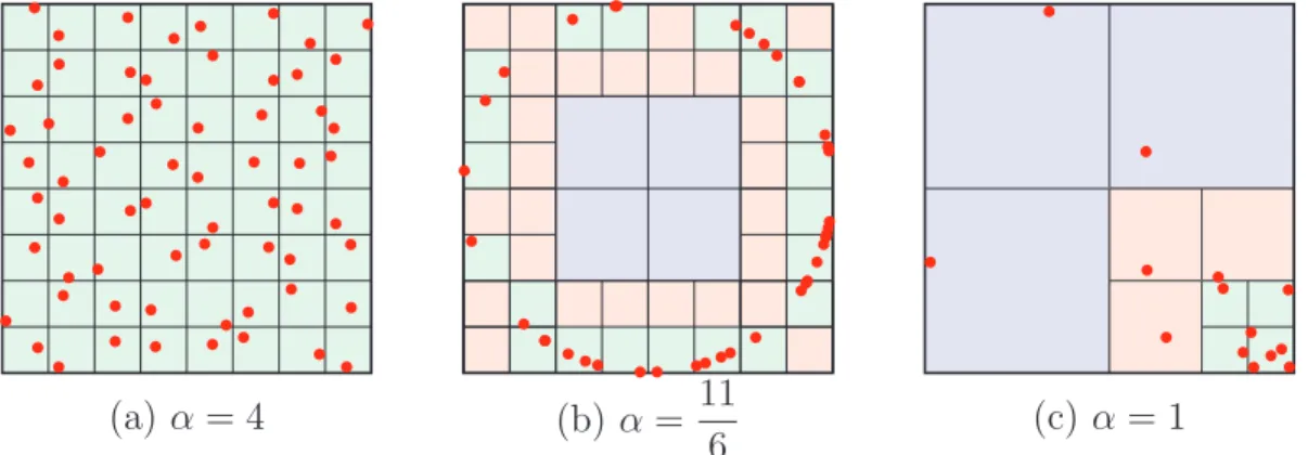
We consider several concrete examples as shown in Figure 3.1. In the figure, three levels of
refinement have been carried out for each case and the corresponding values ofαare computed.
In Figure 3.1 (a), the particle sampling is uniform, and α= 4 reaches the upper bound. As a
result, the depth of the tree is the shortest. In Figure 3.1 (b), α value is in the range of (1,4)
and therefore the depth of the tree will beO(logN). However, sinceαdoes not reach the upper
bound, the depth will be longer than that in case (a). In Figure 3.1 (c), α = 1 reaches the
lower bounds. In this worst case, we can expect the depth of the tree to be O(N). A second
examination suggests that the usual definition for the computational domain is not suitable in
this case. It should be considered as two clusters of particles in order to reduce the length of
the critical path. More precisely, suppose that starting from level l∗, the value of α falls into
(1,2d] for all the levels l ≥ l∗, then all particles contained in the box to be refined at level l∗ should be considered as one cluster while the rest particles form the other cluster.
• • • • • • • • •• • • • • • • • • • • • • • • • • • • • • • • • • • • • • • •
(b) α = 11 6 • • • • • • • • ••• •••
(c) α= 1
• • • • • • • • • • • • • • • • • • • • • • • • • • •• • • • • • • • • • • • • • • • • • • •• •• •• • • • • • • • • • • • •
(a) α= 4
3.2.2
Maximum Concurrency under Dependency Constraints
In this section, we analyze the maximum concurrency potential of FMM subject to dependence
constraints under PRAM architecture according to Bernstein’s conditions [7]. In this process,
we assume that data distribution satisfies the exponential node growth condition.
Given two program fragments Pi andPj, Bernstein’s conditions describe when the two are independent and can be executed in parallel. For Pi, let Ii be all the input variables and Oi the output variables, and likewise forPj. Pi and Pj are independent if they satisfy
Ij∩Oi=∅ (3.2)
Ii∩Oj =∅ (3.3)
Oi∩Oj =∅ (3.4)
Violation of the first condition introduces a flow dependency, corresponding to the first
state-ment producing a result used by the second statestate-ment. The second condition represents an
anti-dependency, when the first statement overwrites a variable needed by the second
expres-sion. The third and final condition represents an output dependency: when two statements
write to the same location, the final result must come from the logically last executed
state-ment.
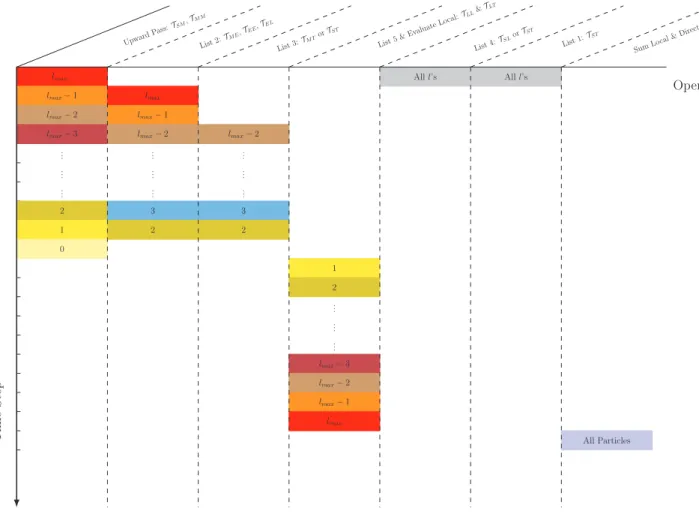
According to Bernstein’s condition, we examine the dependence of the operators involved
in each stage of FMM and produce the maximum concurrency graph as depicted in Figure 3.2.
A detailed explanation is as follows.
First, far-field and near-field operations can start simultaneously from the beginning of the
program since they have independent output sets (write to different memory locations). This
means, generating multipole expansion at level lmax (far-field approximation) and processing list 1 for all childless boxes at each particle location (near-field direct interaction) are executed
in parallel once the program begins.
lmax
lmax−1 lmax
lmax−2 lmax−1
lmax−3 lmax−2 lmax−2
.. . .. . .. . .. . .. . .. . .. . .. . .. .
2 3 3
1 2 2
0 1 2 .. . .. . .. .
lmax−3
lmax−2
lmax−1
lmax
Alll’s Alll’s
All Particles Upward
Pass:T
SM, TM M
List2:
TM E, TEE,
TEL
List3:
TM Tor TST
List5 & Evaluate
Local:
TLL& TLT
List4:
TSLor TST List1: TST SumLocal & Direct Time Step Operations
of the program, namely, processing list 4. There exist two options to process list 4, either by
generating local expansion from particle information usingTSLoperator or by direct interaction usingTST operator. The latter choice can induce potential writing conflicts with the operations related to list 1. However, under the PRAM assumption, it can be avoided by providing
separate storages for the outputs. Doing so can also improve the accuracy of the numerical
results. Recall when adding a set of numbers that differ by several orders of magnitude, it
is more accurate to add the smaller values prior to the larger ones. Analogously, the results
obtained from processing list 1 are larger in magnitude than those obtain from processing list 4
since the particles are further apart in the latter case. Using separate storages, we can calculate
the contribution from each group accurately, hence yielding a better numerical result.
For boxes at levell, we only need their multipole expansions to process lists 2 and 3, which
means these operations can start once the multipole expansions become available. Similar to
processing list 4, there also exist two options to process list 3, either by direct interaction
using TST operator or by evaluating multipole expansion using TM T operator. Under PRAM assumption, the direct interaction operation will not induce any writing conflict. More precisely,
with sufficient resources, generating multipole expansion at level lmax, and processing lists 1 and 4 can be completed in one time unit. Since there exists no box with a non-empty list 3
until levellmax−2 (after two time units), there will be no writing conflict due to applyingTST operator.
As the multipole expansion of a parent box depends on those of its children, the remaining
part of the upward pass is processed sequentially, one level per time unit. Analogously, we
process list 5 (shifting local expansion) and evaluate local expansion for particles in childless
boxes one level per time unit.
In the last step, the results corresponding for near-field (direct interaction) and far-field (
![Table 2.1: Timing results for FMM-Yukawa for 3-digit accuracy with charges uniformly distributed inside the cube [−0.5, 0.5] 3](https://thumb-us.123doks.com/thumbv2/123dok_us/8270460.2190603/43.918.370.580.277.398/table-timing-results-yukawa-accuracy-charges-uniformly-distributed.webp)