Molecular cloud formation in high-shear, magnetized
colliding flows
E. Fogerty
1?, A. Frank
1, F. Heitsch
2, J. Carroll-Nellenback
1, C. Haig
2, M. Adams
11 206 Bausch & Lomb Hall, Department of Physics & Astronomy, University of Rochester, Rochester, New York, 14627, United States 2 3255 Phillips Hall, Department of Physics & Astronomy, University of North Carolina, Chapel Hill, North Carolina, 27599, United States
Submitted 2015 February 28
ABSTRACT
The colliding flows (CF) model is a well-supported mechanism for generating molec-ular clouds. However, to-date most CF simulations have focused on the formation of clouds in the normal-shock layer between head-on colliding flows. We performed simulations of magnetized colliding flows that instead meet at an oblique-shock layer. Oblique shocks generate shear in the post-shock environment, and this shear creates inhospitable environments for star formation. As the degree of shear increases (i.e. the obliquity of the shock increases), we find that it takes longer for sink particles to form, they form in lower numbers, and they tend to be less massive. With regard to magnetic fields, we find that even a weak field stalls gravitational collapse within forming clouds. Additionally, an initially oblique collision interface tends to reorient over time in the presence of a magnetic field, so that it becomes normal to the oncom-ing flows. This was demonstrated by our most oblique shock interface, which became fully normal by the end of the simulation.
Key words: magnetohydrodynamics(MHD) – ISM: kinematics and dynamics – ISM: structure – ISM: clouds – stars: formation
1 INTRODUCTION
The interstellar medium (ISM) is a dynamic environment where material cycles from a warm, tenuous phase to a cold, dense phase and back again. The evolution of the gas through these phases establishes limits on star formation in the galaxy. Understanding the details of such dynamics is crucial as theoretical scenarios for molecular cloud evo-lution (and hence star formation) have shifted away from models based on long molecular cloud lifetimes (i.e. steady states whereτcloud>> τf f; cf. Shu, Adams & Lizano (1987);
Mouschovias (1991)) . Over the last decade or more, evi-dence has grown that instead supports a scenario in which clouds aretransient structures born out of the cold, dense phase of the ISM. For example, starless clouds appear to be scarce, meaning clouds do not slowly evolve towards condi-tions in which star formation begins (Beichman et al. 1986; Dame, Hartmann & Thaddeus 2001). Also, the majority of stars in clouds are, in general, young showing ages<5M yr
(Hartmann, Ballesteros-Paredes & Bergin 2001). This im-plies that star formation begins soon after the cloud itself forms and that clouds are not generally long-lived due to the absence of older stars (Fukui & Yonekura 1998; Palla &
? E-mail:[email protected]
Stahler 2000; Carpenter 2000). Finally, high degrees of hier-archical structure in molecular clouds should have short life-times due to star-star scattering or tidal interactions (Lada & Lada 1995; Eisenhauer et al. 1998; Beck, Kelly & Lacy 1998).
While observational support for short cloud lifetimes has grown steadily, we note that scenarios invoking rapid cloud and star formation are not new (Hunter 1979; Lar-son 1981; Hunter et al. 1986; Ballesteros-Paredes, Hart-mann & V´azquez-Semadeni 1999a). Given the complexity that comes with a dynamical theory of molecular cloud evo-lution, however, exploring the full dynamics of these sce-narios depends heavily on high performance computational methods. One scenario that generates transient molecular clouds and whose exploration has been possible with mod-ern numerical simulations is the ’colliding flows’ model of molecular cloud formation. In this model, molecular clouds are formed in the shocked collision layer between two large-scale colliding streams of gas. Simulations of colliding flows have shown that nonlinear density structures readily form in the shocked collision region between the flows via a va-riety of instabilities (cf. Heitsch et al. (2005) for discussion of the unstable modes). Further, these structures develop column densities high enough for effective UV-shielding, and thus, H2 formation (N ≈ 1−2 cm−2; van Dishoeck
& Black (1988); van Dishoeck & Blake (1998)). Gravita-tional instabilities then cause the turbulent, shocked gas in the dense structures to collapse and form stars. Given the highly dynamical environment, the transition from the beginning of molecular cloud formation to star formation to cloud destruction occurs in roughly a dynamical time (Audit & Hennebelle 2005; Heitsch et al. 2006; V´ azquez-Semadeni et al. 2006; Heitsch et al. 2008), matching obser-vations (Elmegreen (2000); Ballesteros-Paredes & Hartmann (2007), and references therein). The clouds produced in col-liding flows simulations are similar in many ways to those seen in observation.
While colliding flows models tend to be idealized, they are not without motivation. Coherent large-scale streams of gas are plausible in many situations in the ISM, such as, expanding bubbles driven from energetic OB associations and/or supernovae, turbulent motions arising from grav-itational instabilities, density waves in the spiral arms of galaxies, and cloud-cloud collisions (Hartmann, Ballesteros-Paredes & E. 2001; Inutsuka et al. 2015). Observational ev-idence supporting these various scenarios, as well as their association with molecular cloud formation, takes a number of forms. Atomic inflows surrounding molecular gas have been observed in Taurus (Ballesteros-Paredes, Hartmann & V´azquez-Semadeni 1999b) and other molecular clouds (Brunt 2003). Looney et al. (2006) show that the active star forming molecular cloud core in BD +40 4124 likely arose from cloud-cloud collisions (a localized version of a collid-ing flow). Molecular clouds have been found at the edges of supershells (Dawson et al. 2011, 2013), which are a form of colliding flows driven by multiple supernovae.
If molecular clouds form via the accumulation of gas on dynamical timescales (Hartmann, Ballesteros-Paredes & Bergin 2001), then magnetic fields are expected to be dy-namically important on similar timescales. Some colliding flows simulations have studied the role of magnetic fields in molecular cloud formation (Heitsch et al. 2007; Hennebelle et al. 2008; Banerjee et al. 2009; Heitsch, Stone & Hart-mann 2009; V´azquez-Semadeni et al. 2011; Chen & Ostriker 2014; K¨ortgen & Banerjee 2015). Some of these simulations (Heitsch et al. 2007; Hennebelle et al. 2008; Banerjee et al. 2009) have found power law relations between the magnetic field strength and density, similar to what is seen observa-tionally, i.e.B∝nk, where 1/2< k <2/3 forn >100cm−3,
and k = 0 for n < 100 cm−3 (Troland & Heiles 1986; Crutcher 1999; Crutcher et al. 2010; Tritsis et al. 2015). The inclusion of fields in the models also reduces the star for-mation rates to values more in agreement with observations (V´azquez-Semadeni et al. 2011; Chen & Ostriker 2014). Such a reduction has been claimed to result from lower degrees of turbulent substructure found in the simulations (Heitsch et al. 2007; Hennebelle et al. 2008; Heitsch, Stone & Hart-mann 2009; Chen & Ostriker 2014).
While the colliding flows model has proved useful for un-derstanding transient molecular cloud formation, the great majority of work has focused on head-on collisions, with no obliquity in the initial shocks formed in the flow. It is there-fore worthwhile to explore the consequences of allowing the flows to interact at an interface initially inclined relative to incoming velocity vectors. Strong shear in the interaction region can lead to stretching of embedded field lines and the possible generation of turbulence from KH modes. The role
of shear in molecular cloud and star formation has begun to be investigated numerically. Hydrodynamic simulations by Rey-Raposo, Dobbs & Duarte-Cabral (2015) show that clouds can inherit shear velocity fields during their forma-tion in spiral arm galaxies, and that these shear flows impair subsequent star formation. K¨ortgen & Banerjee (2015) find that varying the intersection angle of magnetized colliding flows reduces the star formation efficiency of the gas. This was attributed to a post-shock shear flow disrupting the for-mation of high density structures.
Continuing along these lines, we address the role of shear and magnetic fields in molecular cloud formation, with a focus on the bulk dynamics of the flow. Shear is generated in our models by keeping the flows parallel and varying the angle of the collision interface. We present four adaptive mesh simulations, at a peak resolution of 0.05pc, varying the collision interface from a normal incidence to highly in-clined. All of our simulations include a uniform magnetic field aligned with the flows to simulate idealized ISM condi-tions. We also include self gravity and time-dependent cool-ing. We present our numerical model in Section 2, our results in Sections 4-9, and our discussion in Section 10.
2 NUMERICAL MODEL
We conducted our simululations using AstroBEAR1 (Carroll-Nellenback et al. 2013), a publicly available, mas-sively parallelized, adaptive mesh refinement (AMR) code that contains a variety of multiphysics solvers (i.e. self-gravity, magnetic resistivity, radiative transport, ionization dynamics, heat conduction, and more). Our setup was of two, 40pcdiameter cylinders colliding in a 3D domain un-der the influence of gravity, magnetic fields, and cooling (Fig. 1). Gravity and cooling source terms were solved using a Strang-split corner upwind transport (CTU) scheme that was 2nd-order accurate in time. This was combined with a directionally unsplit CTU scheme for the 3D ideal magne-tohydrodynamics (MHD) equations, using the HLLD Rie-mann solver. Gravitational interactions included both the self-gravity of the gas, as well as the gravitational accelera-tion due to sink particles, which were implemented following Federrath et al. (2010a). To solve Poisson’s equation for the gravitational potential of the grid, AstroBEAR usesHYPRE2
(Falgout & Yang (2002); see the appendix in Kaminski et al. (2014) for a description of AstroBEAR’s self-gravity algo-rithm).
A uniform magnetic field was initialized everywhere in the box, parallel to the flows. The field was initially dynam-ically weak, withβ= 10 andβram ≈38 at the start of the
simulations (βis the ratio of thermal to magnetic pressure, andβramis the ratio of ram to magnetic pressure). The field
had an initial strength ofB= 1.3µG, which is at the lower end of current ISM magnetic field estimates (Beck 2001; Heiles & Troland 2005). Cooling and heating were included using a parametrized cooling curve adapted from Inoue & Inutsuka (2008) to include the effects of UV shielding. The
1 https://astrobear.pas.rochester.edu/trac/
Figure 1. Model diagram. Two oppositely driven cylindrical flows intersected at an angleθ, rotated about they−axis. The in-terface was perturbed with a random sequence of sine waves. The flows were homogeneous and embedded in a stationary, uniform ambient medium of the same density and pressure. The setup was initialized with a uniform magnetic field inx, parallel to the direction of the colliding flows.
modification allowed the gas to cool toT = 10Kfor densi-ties greater thann >1000cm−3 (Ryan & Heitsch in prep).
Our simulations tracked the formation of gravitationally collapsed objects (sink particles) which were created only after a series of checks had been satisfied, e.g.,
(i) a cell and surrounding region was Jeans unstable (ii) the center cell (i.e. location of potential sink) in this Jeans unstable region was collocated with a gravitational potential minimum
(iii) the surrounding region was exhibiting a converging flow into this center zone
etc., as given in Federrath et al. (2010a). These checks en-sured that sinks formed only when appropriate, i.e. when a region would go on to form a gravitationally bound object if better resolution were available. The simulations had 5 levels of AMR, giving a finest cell size of ∆xmin= 0.05pc.
Given this resolution, we identified single sink particles as protoclusters rather than protostars. We will therefore use the words ’sink’ and ’protocluster’ interchangeably.
Sink particles interacted with the gas (and other sinks around them) through gravitational interactions, and the ability to accrete surrounding material. They remained in-dividual objects throughout the course of the simulation (i.e. did not merge), and did not provide any form of energy or momentum feedback into the surrounding medium (i.e no winds or radiation). Gas around a sink particle was accreted only when the density in the surrounding zones exceeded a given threshold, dictated by the Truelove condition (Tru-elove et al. 1997),
λJ>4∆xmin (1)
where λJ is the cell-centered Jeans length. Then, only the
excess gas was removed (Federrath et al. 2010a).
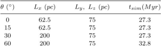
Table 1.The suite of simulations.θ,Lx,Ly,Lz, andtsimdenote
the inclination angle, box dimensions, and final simulation time, respectively. The box size was increased in two of the runs to accommodate the steeper angle. The final simulation time was extended in theθ= 60◦case to check for sink particle formation.
θ(◦) Lx(pc) Ly, Lz(pc) tsim(M yr)
0 62.5 75 27.3
15 62.5 75 27.3
30 200 75 27.3
60 200 75 32.8
The suite of simulations consisted of four runs, each with a different orientation of the collision interface, spec-ified by the inclination angle θ (Table 1). The inclination angle was varied betweenθ= 0◦ andθ= 60◦, i.e. between a head-on and highly inclined collision. This translated into the difference between a normal shock at the collision layer and an oblique shock. All parameters for the present suite of runs were the same as the ’smooth’ model of Carroll-Nellenback, Frank & Heitsch (2014), with the exception of the magnetic field and the variation of the collision inter-face (the smooth run was a hydro, head-on collision). We will therefore compare theθ = 0◦ run to the smooth run to study the effect of the magnetic field alone. Hence, the smooth run from here on out will be called the ’hydro version of theθ= 0◦ case’ (or, the ’hydro run’, for short).
The flows were injected into a stationary ambient medium at a velocity of v = 11 km s−1 and an isother-mal mach ofM = 1.5. The mean molecular weight was set to µ = 1.27, and the adiabatic exponent toγ = 5/3. The gas was initially in thermal equilibrium at a uniform num-ber density ofn= 1 cm−3, corresponding to the (linearly) stable, warm neutral medium (WNM) phase of the cooling curve. This set the thermal pressure and temperature ev-erywhere inside the box to bePtherm k−B1= 4931K cm
−3
, andT = 4931K, wherekB is the Boltzmann constant. The
ram pressure of each flow wasPramk−B1= 18,500K cm
−3
, giving a total mass flux into the collision region ofMf lux≈
886MM yr−1.
As in previous simulations, the collision interface was seeded with a set of random sinusoidal perturbations to ex-cite the nonlinear thin shell (NTS) and Kelvin Helmholtz (KH) instabilities (Heitsch et al. 2006; Carroll-Nellenback, Frank & Heitsch 2014). These perturbations had a maxi-mum amplitude ofA= 2pc, spectral indexα=−2.0, and maximum wave numberkmax = 16 pc−1. Boundary
condi-tions on the box were set to inflow-only on the faces where the flows were injected, and extrapolating on all other faces. The boundary conditions for the gravity solver were set to multipole expansion.
The simulations were initialized to 3 levels of AMR, with the finest cells centered on the collision interface within a cylindrical volume 40pcin diameter and 20pclong, and the coarser meshes nested outwards from there. This made for an initial effective resolution of ∆xef f = 0.2 pc. Two
additional levels were triggered throughout the simulation based on gradients in the fluid variables, as well as resolution of the local Jeans length (λJ), such that if a cell’s λJ was
smaller than 64 zones on that cell’s level, another level of AMR would be added. This brought the finest cell size to
∆xmin= 0.05pc, as previously stated. The final simulation
time for all of the runs was tsim = 27.3 M yr, with the
exception of theθ= 60◦. This was the only run that did not form any sink particles by this time, and so was extended out untiltsim= 32.8M yr.
In what follows, our analysis will focus on the θ = 0, 15, and 60◦cases, as theθ= 30◦ case did not significantly differ from theθ= 15◦case.
3 GENERATING SHEAR VIA AN OBLIQUE COLLISION INTERFACE
The jump conditions across an oblique, 1D, shock-bounded slab convert initially intersecting velocity vectors into a shear flow field. As a measure of this shear for our setup here, we produced mass weighted histograms of the magni-tude of the vorticity (||∇ ×~v||) in cylindrical analysis re-gions centered on the collision region. Each of these ”hockey pucks” encompassed the corresponding collision region by tracing the collision interface and extending out to 5pcon either side of the interface. They were normalized to con-tain the same amount of mass (1,000M). Histograms were generated at t = 1M yr, which is approximately the time it would take a post-shock sound wave to travel from the center of the CF cylinder to the outer boundary.
As can be seen in Fig. 2, lower shear runs (i.e., θ = 0−15◦) have significantly more mass at lower vorticity (||∇×
~
v||<100), than at higher. As the collision angle increases toθ = 30◦, we see two changes occur. First, the amount of mass at||∇ ×~v|| ≤1 decreases considerably. Second, more of the mass moves to higher vorticity. As the collision angle steepens to 60◦, this trend strengthens. For the θ = 60◦ case, there is neglibible mass at the lowest||∇ ×~v||. That is to say, nearly all of the mass has acquired vorticity in this run. Moreover,mostof the mass has acquired high vorticity (||∇ ×~v||>10).
Thus, as the inclination angle increases, more vortic-ity is generated in the collision layer. This vorticvortic-ity can be associated with the solenoidal mode of the post-shock tur-bulence (Federrath et al. 2010b). Turbulent solenoidal fluid motions are efficient in providing support against collapse. Compared to compressive modes of turbulence, Federrath & Klessen (2012) show that solenoidal modes greatly reduce the star formation rate in turbulent, magnetized clouds. The passage of gas through the oblique shocks of our simula-tions thus transforms the compressive nature of the flows into solenoidal. In this way, our higher shear cases should exhibit greater degrees of turbulent support.
4 MASS-TO-FLUX RATIO
Before we present the results of the simulations, we will first discuss some general issues associated with gravitational sta-bility and magnetic fields that are relevant to our studies. We begin with the critical mass-to-flux ratio (M2FR) of cylindri-cal uniform flows. The M2FR compares the relative strength of the magnetic field to gravity. It does not take into account other forces which oppose gravity, such as thermal or ram pressure forces. The M2FR is given by,
Figure 2.Mass-weighted vorticity histograms att= 1M yr. The legend gives the inclination angle (◦) of the given run. Each of the histograms were binned from a cylindrical analysis region centered on the given collision interface (see text), and were normalized to contain 1,000 M. Units are scale-free, where the scale factors are given byM M−1= 100,ll−1(pc) = 1,vv−1(cms−1) = 8091.
µcrit=
Σ
B ≈
1 √
4π2G (2)
where Σ is the mass column density andB is the magnetic field threading the cylinder (Nakano & Nakamura 1978). Equation 2 can be rearranged for the critical lengthof the cylinder. In terms of typical ISM values this is given by,
Lcrit≈470pc(
B
5µG) ( n cm−3)
−1
(3)
where n is the number density (V´azquez-Semadeni et al. 2011). For the initial WNM values of our flows (n= 1cm−3,
B= 1.3µG), Eqn. 3 gives a critical length of,
Lcrit,W N M≈122pc (4)
for the WNM component of the gas. Using this, we can ask whether we would expect the warm gas to be magnetically supercritical. We first have to define a length scale over which we will check stability. Naturally this would be the collision region, as this is where the molecular clouds will be forming. As we will see, the width of this region (Lcoll) is
on the order of 10pc. This means that over the length scale of the collision region, the flow would besub-critical. That is, givenLcrit>> Lcoll, the magnetic field, at least initially,
should be strong enough to withstand gravity.
Ncrit≈1.45×10²¹(
B
5µG)cm −2
(5)
(V´azquez-Semadeni et al. 2011). For simplicity, we imagine the collision region to be initially massless. Its column den-sity as a function of time is then,
N(t) = 2nvt (6)
where v is the speed of the flows. Equating this to Eqn. (5) and solving for t gives the timescale for the collision region to become magnetically supercritical:tcrit≈6M yr.
Thus, the collision region is expected to very quickly (i.e.
tcrit<< tsim) become magnetically supercritical. While this
is a crude estimate, when taken in an average sense (over the collision region) it implies that themeanfield is unable to support the collision region against collapse. However, despite this prediction of a weak field, we did not see a large-scale, global collapse occur in our simulations. This, we will argue, was due to the kinetic energy of the flows themselves, which also prevented global collapse in the hydro version of theθ= 0◦case (Carroll-Nellenback, Frank & Heitsch 2014), rather than the magnetic field. Thus, the M2FR should be used with caution for estimating global stability within the colliding flows model.
We next consider smaller scales associated with the cold, dense phase out of which molecular clouds form. The cold neutral medium (CNM) in our simulations had number densities of approximatelyn≈500cm−3. For the same ini-tial uniform magnetic field, the critical length for the CNM is,
Lcrit,CN M≈0.2pc (7)
As we will see, column density structures associated with the CNM were typically much larger in width than this. Thus, widespread localcollapse (i.e. over length scales associated with the cold component of the gas) might be expected to occur in our simulations.
However, we did not see widespread local collapse. Clearly, the magnetic field assumption in the M2FR calcu-lation was in error. Turbulent instability behind the shocks would have deformed the magnetic field, thereby producing strong field fluctuations. We suspect that field amplification within the cold, dense gas inhibited collapselocally, and that only after the excess magnetic energy was lost (e.g. through numerical reconnection), could collapse proceed. Thus, we expect the cold clumps were actually largelysub-critical and that this could have been shown through a more rigorous calculation of the local M2FR. While such a calculation was beyond the scope of this paper, others have worked on cal-culating the local M2FR in simulations (e.g. Banerjee et al. (2009); V´azquez-Semadeni et al. (2011); Chen & Ostriker (2014)).
Thus, in what follows we will be concerned with issues of local vs. global collapse and the mechanisms by which other processes, such as, turbulence and field amplification, can inhibit collapse. In particular, we must consider that for large values of the inclination angleθ, post-shock flows can retain a significant fraction of their pre-shock velocity. As shear leads to turbulence, we expect the turbulent velocity
to be some fraction of the incoming velocity (vturb ∝f vo).
If turbulence provides support to the cloud against collapse, then we would expect enhancements of the local Jeans length due to turbulence (λturb) to be of order,
λturb
λJ
∝ f vo
cs(x)
(8)
wherecs(x) is the local sound speed. Thus, depending on the
fraction of inflow velocity retained by the turbulence, we ex-pect the collision region in flows with shear to be more stable to collapse than those without shear. In addition, any degree of turbulence will produce local field amplifications (i.e. ad-ditional support against collapse), which as stated, was not accounted for by the M2FR analysis presented above.
5 PROTOCLUSTER FORMATION AND EVOLUTION
In this section we summarize our principle result by demon-strating how shear and magnetic fields directly affected the star formation in terms of the creation of sink particles. While the sink particles in our simulations had masses that should be associated with clumps (i.e. protoclusters), were we to include higher levels of resolution we would expect the clumps to form cores which would then collapse to form individual stars.
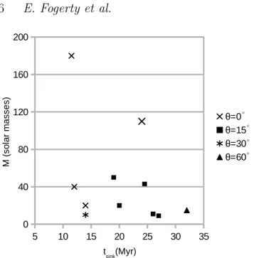
Fig. 3 presents the final masses of the sink particles as a function of their formation time for the various runs. This plot relays three pieces of information that show the effect of shear. First, the total number of protoclusters formed in each of the runsdecreasedwith shear. The number decreased from four protoclusers in theθ = 0◦ case to one in theθ = 30◦ case to zero in theθ = 60◦ case (in the run time given to the other simulations). Only after extending the θ = 60◦ case out another 5M yrdid a protocluster eventually form attsink(θ= 60◦)≈32M yr, as shown in Fig. 2. While this
trend did not hold for the θ = 15◦ case, which formed a couple of low mass protoclusters late in the simulation, it is clear that the initial inclination angle of the colliding flows interface was directly related to the amount of post-shock support against collapse.
Second, higher levels of sheardelayedthe formation of protoclusters. Theθ = 0◦case produced a protocluster by
t ≈ 11 M yr, whereas the θ = 15◦ case did not produce a protocluster untilt≈18M yr. As mentioned above, the (θ= 60◦) was inhospitable enough that protocluster forma-tion was delayed untilt≈32M yr. This shows the various simulations were evolving under different timescales. This can be understood by considering tcrit - the timescale to
acquire enough material into the central region to go mag-netically supercritical. As the inclination angle was varied, the velocity in Eqn. 6 would have becomev0 =vcosθ, due to deflection at the collision interface (i.e. the generation of shear). Thus, the critical timescale for shear environments is related totcritby,
t0crit∝tcrit(cosθ)
−1
(9)
This equation predicts longer timescales for gravitational in-stability in higher shear environments, consistent with the
5 10 15 20 25 30 35 0 40 80 120 160 200 θ=0 θ=15 θ=30 θ=60
tsink(Myr)
M ( so la r m as se s) ◦ ◦ ◦ ◦
Figure 3.Final mass distribution of protoclusters as a function of formation time,tsink. Note, the final simulation time was the
same for theθ= 0,15,and 30◦runs (t
sim= 27.3M yr), but was
longer for theθ= 60◦ case (t
sim= 32.8). Also, mass accretion
was not constant over time, but rather depended on environmen-tal conditions.
increased time to form protoclusters and the overall reduc-tion in protocluster number. Finally we note that while the
θ= 30◦ case does disagree with this result (forming its sin-gle protocluster before theθ= 15◦ case), this sink particle was extremely low-mass despite having ample time to grow. This indicates that while local collapse occurred in the re-gion where the protocluster formed, the shearing motions generated by the initial inclination angle of the interface in-hibited further growth.
Third, shearslowedgrowth of protoclusters, i.e. higher shear cases had lower average accretion rates (< M >˙ =
Mf inal/(tsim−tsink)). For example, consider the two
pro-toclusters that formed at t ≈ 24 M yr. For this pair, the
θ = 0◦ protocluster grew to be ≈ 3× more massive than its θ = 15◦ counterpart. This indicates that the environ-ments surrounding the protoclusters were less bound in the higher shear runs (recall, only gravitationally bound and unstable gas in the surrounding zones can be accreted onto sink particles). The higher accretion rates of the lower shear simulations translated into more massive protoclusters.
The role of magnetic fields on dynamics can also be ex-tracted from Fig. 3, as there was a significant reduction in the number of protoclusters formed in the MHD, no-shear case (θ = 0◦), compared to the hydro version of this run (Carroll-Nellenback, Frank & Heitsch 2014). For the same final simulation time and resolution, the hydro run formed a total of 27 protoclusters compared to the 4 formed in the
θ= 0◦case. Moreover, Carroll-Nellenback, Frank & Heitsch (2014) found differences in the mass distributions of proto-clusters depending on whether there was global or local col-lapse. The present protocluster masses are consistent with the mass distribution of the hydro run, which only exhibited local collapse. Taken together, this demonstrates the local support magnetic fields are providing against collapse, since
Figure 4. Masses of the various sink particles at 1 M yr af-ter their formation with corresponding final masses. Each set of points (early and final mass), is connected by a line. The
θ = 0,15,30,60◦ cases are given by the blue, black, red, and grey lines, respectively. Note that the last sink particle for the
θ= 15◦case is not plotted, as that sink’s lifetime was less than 1M yr. The 60◦ is a single point as that sink lived for exactly 1M yr.
neither the hydro or MHD runs showed evidence of global collapse.
We now turn to comparing the sink particles at a similar evolutionary time. Figure 4 shows the mass distribution of the sink particles at 1M yr post-formation. This time was chosen as it maximizes the accretion time of theθ = 60◦ sink. However, this time loses the final sink of theθ = 15◦ run, which had a lifetime<1M yr. In the figure, each sink’s mass at 1M yr post-formation is connected by a line to the final mass of that sink. This provides a quick reference of the average accretion rates of the sink particles. Figure 4 shows that both the initial peak mass, as well as the average initial mass, decline with increasing shear (focusing on the left-most points of each pair). It is interesting that theθ= 60◦ case seems to contradict this behavior. However, this has to do with the reorientation of the collision interface (discussed in more detail below). By the time this sink particle forms, the initially steep collision angle had become largely normal to the oncoming flows. This would have reduced the degree of post-shock shear, and consequently the amount of support afforded to the surrounding envelope. Thus, theθ= 60◦sink particle was able to accrete at a rate comparable to lower shear runs. Mass-weighted histograms of the vorticity in the collision region for the θ = 60◦ case shows that this has indeed occurred (Fig. 5).
Figure 5. Mass-weighted vorticity histograms for theθ = 60◦ case at early and late times. Solid line is att= 1M yr, dotted is at the end of the simulation (t= 32.8M yr). Each of the histograms were binned from a cylindrical analysis region that was tilted 60◦ and contained 1,000M. Units are again scale-free.
larger. This is why some of the sinks that have formed later in time have grown to be more massive than older sinks.
6 MORPHOLOGY
We now turn to column density maps (CDMs) for a more detailed comparison of the flow evolution. We begin by dis-cussing a morphological artifact common to MHD colliding flows, and then move on to the main morphological features of the flow.
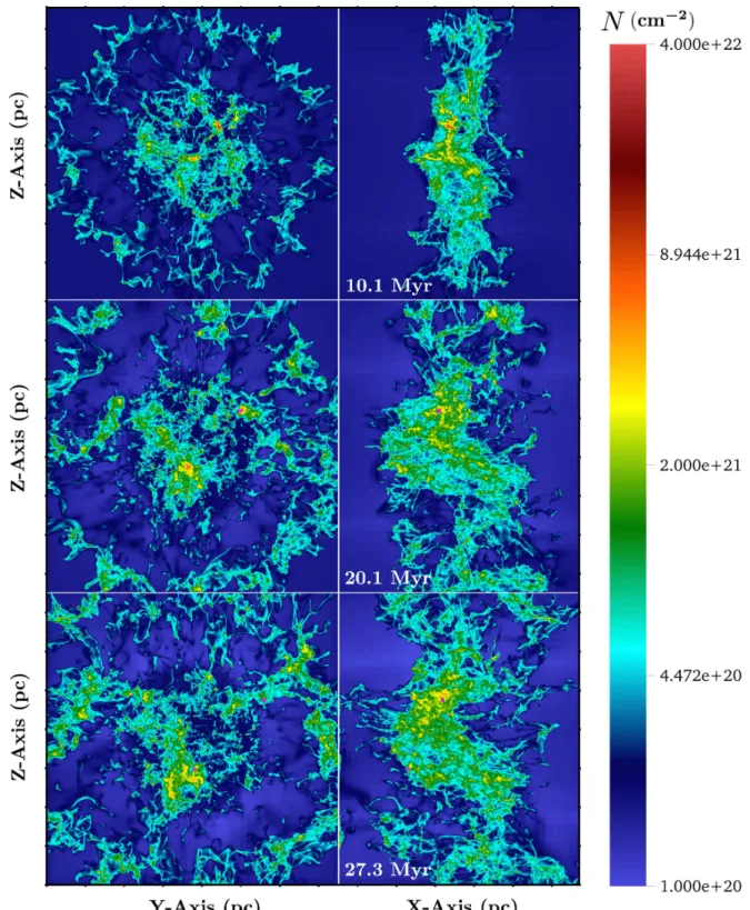
Column density maps of the θ= 0◦case are shown in Fig. 6. As can be seen in the left hand panel, there is a large, ring-like structure surrounding the flows. This ring is an ar-tifact of the simplified initial conditions and its formation can be understood as follows. Initializing colliding flows as cylinders naturally produces a region where shocked gas is expelled laterally with respect to the cylindrical axis. Any colliding flows geometry will produce a characteristic two shock structure (one to decelerate each flow), separated by a contact discontinuity. For finite-sized flows, there must also be a region where high pressure post-shock material is driven out of the collision region. Analysis of a similar process in time variable protostellar jets (which, with a change in ref-erence frame are similar to the configuration studied here), shows that lateral motions on the order of the post-shock sound speed (cps) carry material away from the interaction
region along radial streamlines into the ambient gas (Raga 1992). In this way, converging flows along the length of the cylindrical regions are converted into radial flows expanding away from the axis of the cylinders.
When magnetic fields are present, tension forces can re-strict these lateral motions. The length and time scales for this restriction depend both on the field strength and geom-etry. Studies of magnetized time variable jets with strong cooling show that even initially weak toroidal fields can lead
θ
= 0
◦
Figure 7.Streamline plot ofBxandBzcomponents of the
mag-netic field averaged alongy as shown in thex−zplane for the
θ = 0◦ case. Note the bending of the field lines as material is expelled from the collision region (see text for description).
to the collapse of post-shock flows onto the axis (De Colle, Raga & Esquivel 2008; Hansen, Frank & Hartigan 2015). Thus, the ring-like structure present at approximately 30pc
away from the center of the colliding flows can be attributed to the effect of magnetic tension, since it was not seen in our pure hydro case (Carroll-Nellenback, Frank & Heitsch 2014). Such rings were also seen in other MHD colliding flows runs (V´azquez-Semadeni et al. 2011; Banerjee et al. 2009). We note that in the simulations presented here, the initial field was parallel to the colliding flows. Thus, as post-shock gas was driven outward from the interaction region, the flow drove arcs in the magnetic field (Fig. 7) whose tension even-tually halted further expansion, thereby producing a ring of high density material in the collision plane. The position of this ring can be estimated by assuming the ring has reached a steady-state, as we will do next.
6.1 Magnetized Ring Model
To make calculations simplest, we envision the following sce-nario. Att = 0, the magnetic field isB~ =B0xˆforr > R,
where R is the colliding flows radius. For r < R, we take
B = 0. This is a fine approximation, given the field is dy-namically weak within the flows (recall, βram ≈ 38). As
material enters the collision region, it is shocked and then expands away from the collision region, as described above. We approximate this expansion as being spherically sym-metric.
Now, the ram pressure of the ejecta pushes outward on the surrounding low density, magnetized ambient medium. In 2D, this leads to a ’ring’ of flux that moves outward (in 3D, a spherical ’shell’; Fig. 8). This ring has two boundaries, an outer radius,ro, and an inner radius,ri (Fig. 8,bottom
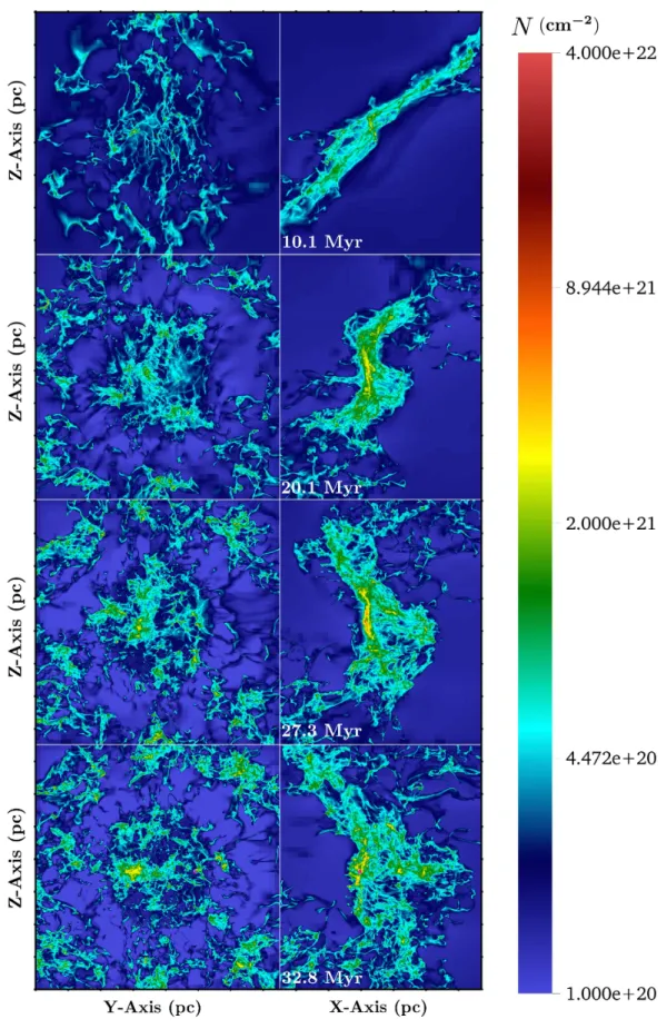
Figure 6. Column density map for theθ= 0◦case. The integration length is the 62.5pcfor the left-hand column and 75pcfor the right-hand column in these and all subsequent column density maps. Sink particles are given as fuchsia points. Each tick mark represents 10pc.
panel). Once this ring comes to steady state, the magnetic pressure atrowill be balanced by the unperturbed, ambient
magnetic pressure,Pmag, which is∝B20. Atri,Pmagwill be
balanced by the ram pressure of the ejecta. We approximate this ram pressure to be the pre-shock ram pressure, given
the low Mach of the flows. Note, we will ignore edge effects near the colliding flows themselves, and instead focus on the dynamics of the ringperpendicularto the flows (Fig. 8,top panel).
Figure 8.Diagram of the magnetic ring model.Top panelshows the incoming flows, spherical post-shock expansion region and corresponding magnetic field arcs, and the direction along which we are integrating the momentum equation (r). Also given is the unperturbed field value (B0), the cylindrical radius of the collid-ing flows (R), and the normal unit vector (ˆn) discussed in the text.Bottom panel shows the ring of high density material (in the mid-plane of the flows) with inner radiusriand outer radius
ro.
ambient (therefore, ignoring gravity and pressure forces), the steady-state ideal MHD momentum equation for the ring is given by,
∇B
2
2µ = B2
µrnˆ (10)
whereµis the magnetic permeability,ris the radius of cur-vature, which we take to just be the distance from the center of the colliding flows to a position in the ring, andnˆis a unit vector normal to the field line that is anti-parallel tor (i.e.
ˆ
n = −ˆr). Defining the radius of curvature in this way is equivalent to assuming the field is being bent along spheri-calarcs. Equation 10 says that in steady state, the magnetic tension of the curved field lines (RHS) is balanced by the gra-dient in magnetic pressure (LHS). Projecting Eqn. 10 onto ther-axis and integrating gives the following expression for
B2(r) in the ring,
B2=B02( ro
r ) 2
(11)
Using this, we balance the magnetic and ram pressures at the ring’s inner radiusri,
B2 0
2µ0
(r0
ri
)2=ρv2(R
ri
)2 (12)
which reduces to,
r0=
p
βramR (13)
Now, the inner radius is where ejected material is being de-celerated, so we wish to find an estimate for this edge of the ring to compare with our simulations. For this, we will use flux-freezing. Equating the flux in the ring at steady state,
θ1=
Z ro
ri
B0r0
r 2πrdr= 2πB0ro(ro−ri) (14)
to the flux in the ring initially,
θ2=
Z ro
R
B02πrdr=πB0(r2o−R
2
) (15)
gives,
ri=
r2o+R2
2ro
(16)
Plugging in forro (Eqn. 13) yields,
ri=R
(βram+ 1)
√ 4βram
(17)
which is approximately,
ri≈
1 2
p
βramR (18)
orr≈3R. As seen from the left hand panel of Fig. 6, this simple model reproduces the ring’s position to within a fac-tor of two.
6.2 Main Features in Column Density
Moving past considerations of the ring, we now focus on the details of the flow in the collision region. Note that the incoming flows corresponded to WNM, which was at a col-umn density ofN ≈2×1020cm−2. After passing through
the shocks, the gas entered the collision region where the thermal instability drove the gas into the CNM state, which the pdfs of Section 8 show was ≈ 500× denser. We iden-tify the different phases in column density loosely, based on morphology and relative mass fraction from previous studies (Heitsch et al. 2007; Hennebelle et al. 2008; Banerjee et al. 2009). In addition, we use the minimumHI column density
for UV-shielding (NHI≈1−2×1021cm−2) to label regions
that have effectively become ’molecular’ (van Dishoeck & Black 1988; van Dishoeck & Blake 1998). Note that to have accurately tracked molecular gas, we would have needed to
include UV shielding in the code. In the images, dark blue regions are the initial WNM, cyan regions are thermally unstable gas, from which the CNM phase and subsequent molecular clouds form (green-yellow), and denser gas (i.e. clumps) within the molecular phase is shown in orange and red.
The structures seen within the interaction region of the
θ= 0◦case (Fig. 6) were morphologically similar to those of the hydrodynamic version of these runs (Carroll-Nellenback, Frank & Heitsch (2014), fig. 2). We note that the degree of heterogeneous or ”clumpy” structure appears to be lower in the present magnetized run. This impression is in line with previous findings for other MHD studies (Heitsch et al. 2007; Hennebelle et al. 2008; Heitsch, Stone & Hartmann 2009; Chen & Ostriker 2014), which find that fields tend to produce larger, more coherent filamentary structures, com-pared to the hydro versions of these simulations.
The first frame of Fig. 6, taken att= 10 M yr, shows the gas shortly before the first protoclusters formed. By the next frame (t = 20 M yr), three protoclusters had formed close enough to each other that two of them overlapped and nearly overlapped the third (as can be seen by zooming in on the figure). The location of these sink particles was off-center from the flow axis, indicating they did not form out of a global collapse mode. Instead, they were within local potential minima, associated with regions of high density gas that condensed out of the background turbulent envi-ronment and had become gravitationally unstable. By the last time panel of Fig 6, another protocluster had formed off-axis, roughly 25pc away. This sink particle was in a large region of high N. Given this sink had the fastest average accretion rate of theθ = 0◦run protoclusters (Fig. 3), this region represented a large and deep potential well. Finally, we note that there was significant widening of the collision region with time, due to the NTS, KH and cooling instabil-ities.
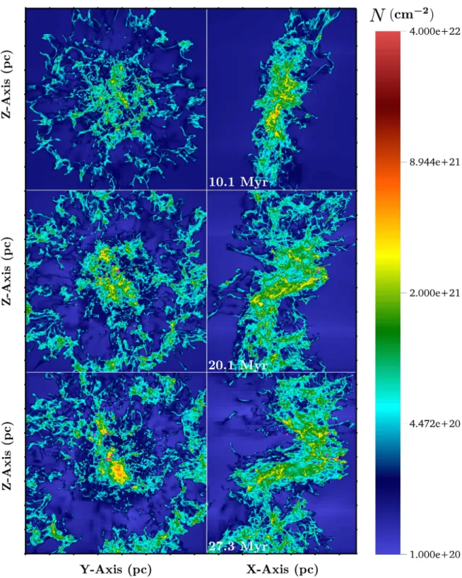
We now shift our attention to column density maps of the θ = 15◦ case (Fig. 9). At t = 10 M yr, the collision region was structurally similar to the 0◦ case, except for regions of lower maximum N (see the left hand column of the plot). Thus, even at low inclination angles, the shear generated by the oblique shocks at the interface disrupted substructure formation to some degree. However, the flows were capable of assembling some localized structures dense enough to become molecular by this time.
Byt= 20M yr, the first protocluster can be seen, hav-ing formed at tsink ≈17 M yr. It is located near the axis
as seen in the left hand panel of Fig. 9, but off-center, in one of the NTSI nodes as seen in the right-hand panel. Over time, the fingers of the NTSI grew, and byt= 27.3M yrthe instability had become ’z-shaped’, with a large component aligned with the flow axis. Also by this time, four addi-tional protoclusters had formed. Two of these were in the same NTSI node mentioned above, and the other two were roughly 10.2 and 21.9pcaway, near the edge of the cylin-der. The positions of all of these sink particles was again consistent with local instability being triggered in the flow. Finally, we discuss the extreme θ = 60◦ case, which exhibited very different behavior than the other runs. In particular, we found that the initial steep angle of the col-lision interface reoriented over time and became normal to
the incoming flows. Animations3 of the runs suggested the
reorientation was due to perturbations at the collision inter-face seeding the NTSI. However, field line tension may have also played a role, as a similar, albeit weaker realignment is seen in the hydro version of this run (Haig & Heitsch in prep). The reorientation appears to begin in a region where the flow was nearly normal to the surface of an NTSI node (see the right panel of Fig. 10 att = 10.1M yr). Because of the high angle of the collision interface, most incoming material was deflected by the oblique shocks to flow parallel along the shock face. The NTSI node created a local dis-tortion of the shock, allowing oppositely driven material to meet at lower obliquity. The gas behind this stronger shock had higher thermal pressure and began expanding in the (y,z) plane. This expansion increased the area of the low obliquity regions of the flow, which led to more high pres-sure post-shock gas as seen byt= 20.1M yr(Fig. 10, right). In this way, it appears the initially highly oblique shock re-gion was transformed into a shock that was more normally directed, relative to the incoming flows. By t = 32.8, the shock had become nearly fully normal.
We conclude with comments on the general character-istics of theθ = 60◦ collision interface. First, the collision region was less dense than in the other runs att= 10.1M yr
(Fig. 10, left). This suppression of growing high density re-gions arose from the strong shear. Incoming material was sharply deflected away from the axis of the cylinder, and thus less gas accumulated at early times. Second, the col-lision interface was thinner compared to the other runs at early times, because of this deflection of material away from the interaction region. Material streamed out into the am-bient medium, rather than building up along the flow axis. Only byt= 20M yr, given the reorientation of the shocks bounding the interaction region (and corresponding weaker degree of shear), did material begin to accumulate in the collision region (Fig. 10, left). Byt= 32.8 M yr, local col-lapse had set in and a single protocluster is visible on the CDM, again having formed away from the global potential minimum.
7 MAGNETIC FIELDS AND DYNAMICS:β−1 MAPS
We next discuss maps of averageβ−1, which were generated
by discretely summingβ−1through the grid along the same lines of sight used in the column density maps of the previous section, i.e.,
¯
β−1 = 1
L
i=mx
X
i=1
βi−1dxi (19)
whereL,mx,β−i1, anddxi are the length of the box along
the given dimension, number of cells along that dimension, value ofβ−1at theithcell, and theithcell’s width,
respec-tively.
Beginning with theθ = 0◦ case, field amplification as-sociated with the radial ejection of gas from the collision
Figure 9.Column density map for theθ= 15◦case. Sink particles are given as fuchsia points. Each tick mark represents 10pc.
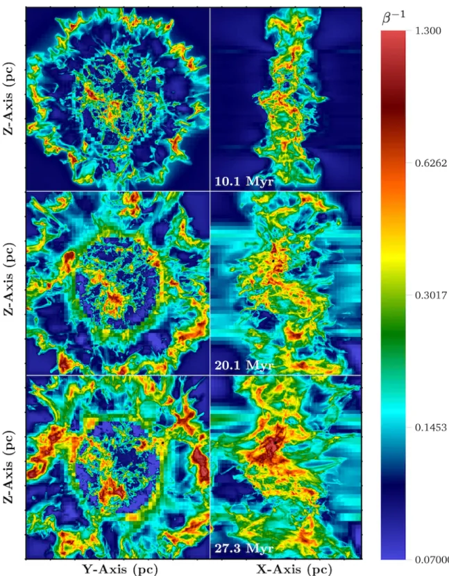
region (discussed in Section 6) produced a ring of high av-erageβ−1 at r ≈30 pc (Fig. 11, left). Additionally, there was another, inner ring present fromt= 10.1M yron at a distance of r≈15pcfrom the center of the colliding flows that did not appear in the CDMs. This ring was not con-tained in the collision region itself, as can be seen from the right-hand frames of Fig. 11. Rather, it stretched down the length of the cylinder, peaking in brightness near the outer
edge. This indicates it was generated by the strong shear present at the boundary between the colliding flows and the stationary ambient medium. This shear layer would have caused strong cooling and therefore a decrease in thermal pressure (hence the increasedβ−1 along this boundary).
Looking down the barrel of the flows att= 10.1M yr
(Fig. 11, left), there are regions inside of the collision region where averageβ−1 had increased above its initial value of
Figure 11.Averageβ−1map for theθ= 0◦case (see Eqn. 19 for definition). Sink particles are given as black points. Each tick mark represents 10pc.
β−1 = 0.1. A glance back at Fig. 6 shows these regions are
co-located with regions of high column densityN. In some of these regions, average β−1 had increased by a factor of
10 or more. Since this material is associated with the CNM phase (as discussed in Section 6), its thermal pressure was
at least equal to its initial value (cf. Section 8). Thus, in order forβ−1to have increased by this amount, the magnetic pressure must have increased by a factor of 10 or more. This supports that the field was being strongly amplified in the high density gas.
In addition, we see regions where average β−1 was re-duced below its initial value. These ’voids’ (shown in the lowest color on the color bar) generally correspond with re-gions of lowN. Since flux freezing implies the accumulation of flux is co-extensive with regions of high density, the voids were formed as material was swept away by both turbulence and the collapse of gas into neighboring potential minima. In other words, voids are associated with regions that have a net positive ∇ ·v. Thus, regions of low N should not be strongly magnetized, consistent with the voids in Fig. 11. As the simulation evolved, there was an increase in the size of both the magnetic voids, as well as, regions of high average
β−1.
The ramifications of magnetic fields on the dynamics of the flow were already discussed in Section 5. The presence of high averageβ−1 regions co-located with regions of high
N support that magnetic fields suppressed star formation
locally. This is further supported by the location of forming protoclusters. As seen in thet= 20.1 and 27.3M yrpanels, protoclusters formed away from regions of highest average
β−1. That is, protocluster formation was inhibited where the field was the strongest. Instead, protoclusters formed where the gas was dense, but averageβ−1.0.6.
Average β−1 maps of the θ = 15◦
case (Fig. 12) are similar to the case with no shear. Regions of high average
β−1are associated with highNstructures. There was also a similar formation of magnetic voids. The shear angle present in these runs does, however, leave a signature in the aver-age β−1 maps early in the simulation. Looking down the
axis of the flows at t= 10.1M yr, it is evident that there are weaker regions of enhanced averageβ−1 (Fig. 12, left).
This likely occurs because of the way incoming flows were redirected away from the axis, due to the oblique shocks. Whereas material was driven away from the collision region with radial symmetry in the no-shear case, material here picked up positive and negative vz components across the
contact discontinuity. The field lines threading the interac-tion region must have therefore undergone a local stretching and may have been shorted out by numerical diffusion. This is in contrast to the large scale arcs of field which formed in the purely radial flows of theθ= 0◦case.
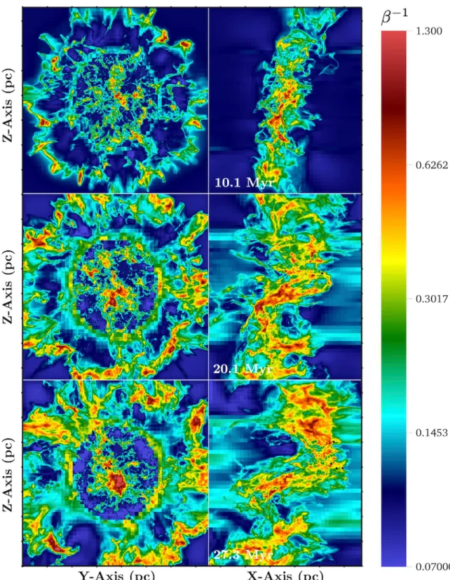
Fig. 13 shows a very different set of averageβ−1 maps for theθ= 60◦case. First we note that projected along the axial view we see almost no regions of high averageβ−1. This is because the interaction region remained quite thin early on as gas passed through the oblique shock and was quickly shunted away from the central region. When seen from the side, however, (Fig. 13, right) we do find significantly higher values of average β−1 in the collision region. This reflects both the projection through the thin interaction region, as well as the strong local field amplification that occurred due to the shear. Field lines must have assumed a ”z” shaped
configuration as gas moving from the left on one side of the contact discontinuity was driven upward by the oblique shock it encountered, and gas moving from the right on the other side of the contact discontinuity was driven downward by the oppositely oriented oblique shock it encountered.
Note that as the collision region reoriented from t = 20.1 M yr onward (cf. Section 6), more material and field collected inside of the interaction region in the same man-ner as was discussed in the lower shear cases. This accounts for the increased regions of high averageβ−1 seen in the left
hand side of Fig. 13 at later times, although overall these regions were much smaller than their lower shear counter-parts.
8 THERMODYNAMICS - PROBABILITY DISTRIBUTION FUNCTIONS
We now discuss the thermodynamic evolution of the gas as it was first shocked in the flow collision and then cooled into a cold, dense state, which could then undergo further compres-sion (or expancompres-sion) due to gravity and/or magnetic fields. The probability distribution functions (pdfs) in this section give the amount of mass at a given pressure and number density. They-axis gives both scaled magneticandthermal pressure (marked by the color and gray scale, respectively), and thex-axis gives number density n (cm−3). Isotherms are straight lines of slopem= 1 on these pdf log-log plots, and increase in temperature from right to left.
We begin with theθ= 0◦run. The thermal pressure dis-tribution (i.e.grey-scale pdf, Fig. 14) in this and the remain-ing runs was identical to previous collidremain-ing flows studies. Namely, gas was shocked and heated as it entered the colli-sion region and via the thermal instability, cooled down until it reached the equilibrium curve. For a more detailed discus-sion of the dynamics relayed by the thermal pressure pdf, we refer the reader to previous work (e.g. Carroll-Nellenback, Frank & Heitsch (2014)). Presently, we consider the simulta-neous thermal and magnetic evolution of the gas as shown by overlaying the Pmag, n pdf in color. Note, however, it
is not always possible toexactlycorrelate values in one pdf with values in the other (i.e. to simultaneously know the
Pthermof a givenPmag, ncombination).
As can be seen in Fig. 14, most of the mass at low densities (i.e. near logn= 0) hadβ >1, consistent with the notion of magnetic voids discussed in Section 7. This follows from comparing thePmag distribution with thePtherm
dis-tribution at these densities. While the disdis-tribution ofPmag
had a much higher spread, this spread was mostly below thePtherm distribution. In contrast, gas at higher densities
(logn > 2.5) was mostly on top of the equilibrium curve, implying most of the densest gas had β < 1. This is in agreement with the densest gas having had enhanced mag-netic support (and thus greater support against collapse), as was also discussed in Section 7. Despite the spread in
Pmag at these highn, the gas was entirely atT = 10K, as
thePthermdistribution was constrained to lie on the
equilib-rium curve at these densities. Lastly, thePmag,npdf tended
Figure 12.Columnβ−1 map for theθ= 15◦case. Sink particles are given as black points. Each tick mark represents 10pc.
Figure 13.Columnβ−1map for theθ= 60◦case. The single sink particle is given as a black point. Each tick mark represents 10pc.
on this log-log plot would correspond to a power law rela-tionship similar to what is observed in other work (Heitsch et al. 2007; Hennebelle et al. 2008; Banerjee et al. 2009).
Now we discuss the dynamics attributable to these var-ious features of the Pmag, n pdf. As the simulation
pro-ceeded, turbulence at the collision interface (produced by the KH and NTS instabilities) generated magnetic field fluctu-ations. Reconnection diffusion, effective at removing excess magnetic energy from magnetized, turbulent flows
(Lazar-ian, Santos-Lima & de Gouveia Dal Pino (2010); see also Klessen, Heitsch & Mac Low (2000); Federrath et al. (2011)), created thelarge(i.e. many orders of magnitude) spread in
Pmagat lown. This spread inPmagpersisted as the gas was
cooled and compressed. Flux-freezing, which accompanied this compression, then led to a sharp increase inPmag, as
Figure 14.Pressure vs. density histograms for theθ= 0◦case. The y-axis gives both the thermal (grey scale distribution) and magnetic (color scale distribution) pressure as a function of number density (the logs of these quantities, that is). The color bar gives the amount of mass at a given pressure and density. The thermodynamic equilibrium curve is given on the plot, as well as the initial magnetic pressure of the flows (bottom horizontal line), ram pressure of the flows (top horizontal line), andT = 10Kisotherm (diagonal line).
within this population was significantly greater than any otherPmag, ncombination of the flow.
As time continued, a high Pmag, n ”tail” of the pdf
formed that, 1) followed the equilibrium curve, 2) was above the ram pressure line of the flows, and 3) only appeared after protoclusters had formed in the flow. Thus, this tail traced gravitational instability in the flow. Most of the mass in the tail was at a β < 1, consistent with the discussion from Section 7 that regions of high density were correlated with regions of highβ−1. Additionally, there was a spread inβ
for the population of gas parcels in this tail, as was also discussed in Section 7. In particular, protoclusters formed in dense enough gas that was at lower average β−1 than the surroundings. Numerical reconnection within this high
Pmag,n tail reduced the local field strength, thus enabling
protocluster formation.
The pdfs for the θ = 15◦ case (Fig. 15) were similar to those for the θ = 0◦ case. The largest difference was the delayed growth of the high Pmag, n tail in the higher
shear run. Thus, the plot offers further evidence that shear suppressed compression in the flows. Eventually collapse was triggered in localized pockets of the flow, allowing gas parcels to begin to climb the equilibrium curve, as seen by t = 20.1M yr. As in the previous case, this coincided with the presence of newly formed protoclusters in the flow.
Keeping in mind the trends discussed previously, Fig. 16 shows an even longer delay in collapse/compression in the highest shear angle case,θ= 60◦. This is evident by the diminished upper-right island of highPmag, nmaterial early
on. It is also shown by the greater delay in the highPmag, n
tail compared to the lower shear runs, which was still not visible byt= 27.3M yr. Only byt= 32.8M yrdid the high
Pmag, ntail emerge in the pdf, again corresponding with the
presence of a newly formed protocluster in the flow.
Table 2.Analysis region for the different runs. Each were cen-tered on the collision interface and had lengths inx,y, andz, given byLx,Ly,Lz. The maximum wavelengthλmax(∝k−min1 )
for each run is also given, which was equal to the longest dimen-sion of the analysis region.
θ(◦) Lx (pc) Ly, Lz (pc) λmax(pc)
0 20 40 40
15 31 40 40
60 90 40 90
9 ENERGY SPECTRA
We next turn to power spectra of the gas in the colli-sion region for kinetic, gravitational, and magnetic ener-gies (Ekin, Egrav,andEmag, respectively), following
Carroll-Nellenback, Frank & Heitsch (2014). To accommodate steeper shear angles, thexdimension of the analysis region increased withθand a 10pcbuffer was added to either side. The dimensions of the analysis region for the different runs are given in Table 2.
Spectra for the different runs are shown in Fig. 17, for three different times. Note, the x-axes in the spectra are equivalent to λmaxλ−1, where λmax is given in Table
2. Thus, each unit on the x-axis represents that fraction of λmax. We include a k−2 line (solid line, red) to
com-pare to the spectra of v2 (dotted-dashed line, black) for
t= 10.1M yr. We do not include thev2 spectrum for other times, as it was largely unchanged throughout the course of the simulations.
As can be seen by the v2 spectrum, gas displayed the Burger’s turbulent spectrum (v2 ∝ k−2) in all of the runs over some range ofk. For the θ = 0◦ case, this was 3< kk−min1 <40, corresponding to length scales of roughly 13pc > λ >1pc. At the lowkend of the spectra, the driving scale of the turbulence is apparent and was on the order of the colliding flows radius (λ≈40pc). At higherk, both
Figure 15.Pressure vs. density histograms for theθ= 15◦case. As before, the y-axis gives both the thermal (grey scale distribution) and magnetic (color scale distribution) pressure as a function of number density (the logs of these quantities, that is). The color bar gives the amount of mass at a given pressure and density. The thermodynamic equilibrium curve is given on the plot, as well as the initial magnetic pressure of the flows (bottom horizontal line), ram pressure of the flows (top horizontal line), andT = 10Kisotherm (diagonal line).
Figure 16.Pressure vs. density histograms for theθ= 60◦case. As before, the y-axis gives both the thermal (grey scale distribution) and magnetic (color scale distribution) pressure as a function of number density (the logs of these quantities, that is). The color bar gives the amount of mass at a given pressure and density. The thermodynamic equilibrium curve is given on the plot, as well as the initial magnetic pressure of the flows (bottom horizontal line), ram pressure of the flows (top horizontal line), andT = 10Kisotherm (diagonal line). Note, the pdfs were similar enough betweent= 20.1 and 27.3M yrthat we do not include thet= 27.3M yrpanel in the figure.
sipation and gravitational collapse limited the inertial range captured in the grid.
The dominant energy on all size scales for all of the runs wasEkin(smooth, black lines), and remained so throughout
the course of the simulations. This was due to the power be-ing generated in the collidbe-ing flows themselves. We note that in the hydro version of theθ= 0◦case (Carroll-Nellenback, Frank & Heitsch 2014), Ekin > Egrav at late times in the
flow on large scales (λ > 10 pc). This indicated a lack of global collapse. The much stronger suppression of Egrav
(fine-dashed lines) in the MHD runs (i.e. Ekin >> Egrav)
shows that large-scale global collapse was also not
occur-ring in the MHD cases. Also,Ekin< Egrav on small scales
(λ <10pc) in the hydro case. This indicated strong local col-lapse was occurring. ThatEkin > Egrav on small scales in
the MHD cases further supports that magnetic fields have impaired local collapse. A diminished degree of local col-lapse occurred in the MHD runs, and only in regions where
Egrav> Emag.
Indeed throughout the runs,Egrav was comparable to
Emag, on most scales. However, in theθ= 0◦case,Egravwas
generally higher thanEmagfor 10< kkmin−1 <100. Note, this
1 10 100 -5 -4 -3 -2 -1 0 1
1 10 100
-5 -4 -3 -2 -1 0 1
1 10 100
-5 -4 -3 -2 -1 0 1 kk-1 min lo g( E ) θ=0○
θ=15○ θ=60○
kk-1
kk-1
min min
Figure 17.Energy spectra for the various runs. Shown are the kinetic (smooth lines), magnetic (dashed), and gravitational energies (fine-dashed) over time (increasing in time from dark to light). There is also av2 line (dotted-dashed line) and correspondingk−2 line (red line) to measure the degree of Burger’s type turbulence in the runs. For theθ= 0−15◦plots, black and gray lines aret= 10.1 and 27.3M yr, respectively. For theθ= 60◦run, black, gray, and light gray lines are fort= 10.1,20.1, and 32.8M yr, respectively.
localized collapse, due to a stronger gravitational field on these scales. Byt= 27.3M yr, there was a slight increase in
Emag relative toEgrav, which may reflect an enhancement
of the field due to compression from gravitational collapse. Theθ= 15◦spectra show similar behavior to theθ= 0◦ case. At intermediate scales, Emag and Egrav were
com-parable. At smaller scales, as gravitational collapse set-in,
Egrav> Emag. The effect of shear in this case did not make
itself readily apparent in the energy spectra.
The spectra for theθ= 60◦case, however, show clearly the effects of imposed shear on the distribution of energies at different scales. At 10 M yr, Emag > Egrav, on all size
scales. In the range of 9< kkmin−1 <90, corresponding now
to size scales of 1 < λ(pc−1) < 10 (cf. Table 2), we see Emag >> Egrav, withEmagapproachingEkinnearkk−min1 ∼
60 (λ ∼ 1.5 pc). Note that this is the only run in which such an equipartition occurred. This enhancedEmagrelative
to Ekin occurred with a simultaneous decrease in power of
Egrav on all scales compared to the other runs. Thus, the
signature of high shear was a relative amplification of the field on protocluster scales, as well as a decrease in Egrav
on all scales, which we attribute to the disruption of dense structures forming in the flow as already discussed. Only by the end of the simulation (t= 32.8M yr) didEgravbecome
comparable with the energy locked up in the magnetic field (which was itself comparable toEkin). Thus, the spectra are
consistent with the formation of a sink particle at late times.
10 DISCUSSION
We have presented 3D, adaptive mesh refinement simula-tions of magnetized, shear colliding flows including self-gravity, sink particles, and cooling. Feedback was not in-cluded in the present work and thus our simulations only fol-lowed the formation and early evolution of molecular clouds. The simulations were of two colliding flows, intersecting at an inclined interface under a dynamically weak magnetic field. The inclined interface was used to generate shear at the collision layer, and was varied from not-inclined
(nor-mal incidence of the colliding flows) to highly inclined. As molecular clouds are unlikely to form from perfectly head-on collisions between two large-scale streams of gas, breaking the symmetry of the collision interface in this way was a previously unexplored next step in the colliding flows model exploration. The purpose of this set of experiments was to study the effect of shear on molecular cloud formation in magnetized colliding flows.
Our work has shown that shear, imposed by an inclined collision interface, impacts cloud dynamics and reduces pro-tocluster formation. In particular, as shear increased (i.e. the inclination angle steepened), it took longer to form proto-clusters, they formed in lower numbers, and they were lower in mass due to diminished accretion rates. These effects are consistent with recent work by K¨ortgen & Banerjee (2015), who found that higher degrees of inclination between collid-ing flows leads to a reduced number of sink particles, as well as a delay in their formation. Additionally, Chen & Ostriker (2014) show that under ideal MHD conditions, increasing the angle between upstream colliding flows and the mag-netic field (which, with a change of reference frame is similar to our setup here) decreases the number of gravitationally bound cores that form in the post-shock region.
We also showed that without shear, protocluster for-mation was greatly impeded in the presence of even a weak field (β = 10, βram ≈ 38) alone. This was evidenced by
the stark difference in protocluster number between the no-shear, MHD case (θ= 0◦) and the hydro version of this sim-ulation in Carroll-Nellenback, Frank & Heitsch (2014). More than 5 times as many protoclusters formed in the hydro run (n=27) compared to the MHD run (n=4). This result fits in with other colliding flows studies that have shown magnetic fields impair gravitational collapse. Hennebelle et al. (2008) showed that it takes longer to form self-gravitating objects in MHD colliding flows (aligned field,B0= 10µG), compared
to flows without a field. Heitsch, Stone & Hartmann (2009) also compared colliding flows with and without a magnetic field and found that the degree of post-shock turbulence decreases with a magnetic field. This led to a suppression of dense cores forming in the magnetized cases.
ally, V´azquez-Semadeni et al. (2011) found that increasing the magnetic field strength in colliding flows simulations de-creases the SFE of forming clouds.
To understand the flow dynamics responsible for the weaker protocluster formation, we began by distinguishing between ’global’ and ’local’ collapse, and showed that col-lapse in our simulations was due tolocalizedregions becom-ing unstable, rather than the entire collision region. Indi-cators of local collapse included the positions of sink par-ticles away from the global potential minimum, weak mass ’fall-back’ into the collision region, and power spectra that showed Ekin > Egrav on large scales, but Ekin < Egrav
on small scales (Carroll-Nellenback, Frank & Heitsch 2014). Our results were consistent with these indicators: sinks formed away from the center of the collision region, they had variable accretion rates, and bothEgravandEmag were
<< Ekinon large scales, butEgrav∼Ekin> Emagon small
scales. All of the runs (θ= 0−60◦), as well as the hydro run, exhibited local collapse only (i.e. did not collapse globally). Compared to the hydro run, collapse was weakened in our θ = 0◦ case due to the interplay between the turbu-lent post-shock velocity field and the magnetic field. Turbu-lence in the interaction region introduced distortions to the magnetic field, which produced regions of local field ampli-fication. These were shown to be co-located with regions of high density (Sections 7 and 8). Thus, local collapse had an additional form of support in the MHD case(s) – magnetic support, due to field amplification (see also Banerjee et al. (2009); Heitsch, Stone & Hartmann (2009)). Over time, nu-merical reconnection would have reduced the field strength in these pockets of dense gas (Lazarian, Santos-Lima & de Gouveia Dal Pino 2010; V´azquez-Semadeni et al. 2011; Fed-errath et al. 2011; Chen & Ostriker 2014), thereby allowing highly localized regions to become magnetically supercriti-cal and produce protoclusters (should the gas also be Jeans unstable).
As shear increased in the flows, a higher degree of post-shock turbulent velocity resulted. This disrupted the forma-tion of dense structures in the flow, which further inhibited local collapse and protocluster formation (by locally decreas-ing the M2FR, as well as, increasdecreas-ing the Jeans length). This seemed to be the dominant effect of shear, as we did not find that stronger shear led to greater field amplification. The reasons for this were likely two-fold. While the shear generated by the oblique shocks at the collision interface would have led to greater distortions of the field (Hartmann 2001; Heitsch et al. 2007; Chen & Ostriker 2014), they were also likely shorted out faster in the higher shear cases. Ad-ditionally, given the disruption of high density structures forming in the flow, regions of increased field strength due to flux freezing would have also been diminished. Both the pdfs and spectra (Sections 8 and 9, respectively) support the con-clusion that field amplification did not increase with shear. They do, however, show decreases in high density structures. This is consistent with K¨ortgen & Banerjee (2015), who at-tribute declining sink particle formation to shear disrupting the formation of high density structures.
Lastly, we discussed the large-scale realignment of the collision interface that took place in our highest shear angle case,θ= 60◦. This unexpected result may have arisen from the orientation of an NTSI node with respect to the on-coming flows, as discussed in Section 6. However, tension in
the magnetic field may have also contributed to the realign-ment. This is supported by current work by Haig & Heitsch (in prep), which shows that the steep 60◦inclination angle reorients to alesser degree withouta magnetic field. A re-alignment of the collision interface was also mentioned in K¨ortgen & Banerjee (2015).
ACKNOWLEDGMENTS
We thank Ralph Klesson, Simon Glover, Mordecai-Mark Mac Low, Eric Mamajek, Alice Quillen, and Andy Pon for interesting discussions on the present work. We thank Christoph Federrath and Clare Dobbs for their valuable comments and suggestions, and Bastian K¨ortgen for propos-ing includpropos-ing an early mass distribution of protoclusters. We thank the referee, Robi Banerjee, for his insightful review and recommending a vorticity analysis. We thank the Uni-versity of Rochester’s Center for Integrated Research Com-puting (CIRC) for time on their supercomputers, data stor-age, and visualization at the VISTA collaboratory, and the Texas Advanced Computing Center and XSEDE for com-puting time. Lastly, we thank Rich Sarkis of the University of Rochester for maintaining our data systems. This work was supported by the U.S. Department of Energy through grant GR523126, the National Science Foundation through grant GR506177, and the Space Telescope Science Institute through grant GR528562.
REFERENCES
Audit E., Hennebelle P., 2005, A&A, 433, 1
Ballesteros-Paredes J., Hartmann L., 2007, RMxAA, 43, 123
Ballesteros-Paredes J., Hartmann L., V´azquez-Semadeni E., 1999a, ApJ, 527, 285
Ballesteros-Paredes J., Hartmann L., V´azquez-Semadeni E., 1999b, ApJ, 527, 285
Banerjee R., V´azquez-Semadeni E., Hennebelle P., Klessen R. S., 2009, MNRAS, 398, 1082
Beck R., 2001, SSRv, 99, 243
Beck S. C., Kelly D. M., Lacy J. H., 1998, AJ, 115, 2504 Beichman C. A., Myers P. C., Emerson J. P., Harris S.,
Mathieu R., Benson P. J., Jennings R. E., 1986, ApJ, 307, 337
Brunt C. M., 2003, ApJ, 583, 280 Carpenter J. M., 2000, AJ, 120, 3139
Carroll-Nellenback J., Frank A., Heitsch F., 2014, ApJ, 790, 37
Carroll-Nellenback J. J., Shroyer B., Frank A., Ding C., 2013, Journal of Computational Physics, 236, 461 Chen C.-Y., Ostriker E. C., 2014, ApJ, 785, 69 Crutcher R. M., 1999, ApJ, 520, 706
Crutcher R. M., Wandelt B., Heiles C., Falgarone E., Troland T. H., 2010, ApJ, 725, 466
Dame T. M., Hartmann D., Thaddeus P., 2001, ApJ, 547, 792
Dawson J. R., McClure-Griffiths N. M., Dickey J. M., Fukui Y., 2011, ApJ, 741, 85