Precision calculations of the cosmic shear power spectrum projection
Martin Kilbinger,
1,2‹Catherine Heymans,
3Marika Asgari,
3Shahab Joudaki,
4,5Peter Schneider,
6Patrick Simon,
6Ludovic Van Waerbeke,
7Joachim Harnois-D´eraps,
3Hendrik Hildebrandt,
6Fabian K¨ohlinger,
8Konrad Kuijken
9and Massimo Viola
9 1CEA/Irfu/SAp Saclay, Laboratoire AIM, F-91191 Gif-sur-Yvette, France2Institut d’Astrophysique de Paris, UMR7095 CNRS, Universit´e Pierre and Marie Curie, 98 bis boulevard Arago, F-75014 Paris, France 3Institute for Astronomy, University of Edinburgh, Royal Observatory, Blackford Hill, Edinburgh EH9 3HJ, UK
4Centre for Astrophysics and Supercomputing, Swinburne University of Technology, PO Box 218, Hawthorn, VIC 3122, Australia 5ARC Centre of Excellence for All-sky Astrophysics (CAASTRO)
6Argelander-Institut f¨ur Astronomie, Auf dem H¨ugel 71, D-53121 Bonn, Germany
7Department of Physics and Astronomy, University of British Columbia, 6224 Agricultural Road, Vancouver, BC V6T 1Z1, Canada
8Kavli Institute for the Physics and Mathematics of the Universe (WPI), The University of Tokyo Institutes for Advanced Study, The University of Tokyo,
Kashiwa, Chiba 277-8583, Japan
9Leiden Observatory, Leiden University, Niels Bohrweg 2, NL-2333 CA Leiden, the Netherlands
Accepted 2017 August 10. Received 2017 August 9; in original form 2017 February 20
A B S T R A C T
We compute the spherical-sky weak-lensing power spectrum of the shear and convergence. We discuss various approximations, such as flat-sky, and first- and second-order Limber equations for the projection. We find that the impact of adopting these approximations is neg-ligible when constraining cosmological parameters from current weak-lensing surveys. This is demonstrated using data from the Canada–France–Hawaii Telescope Lensing Survey. We find that the reported tension withPlanckcosmic microwave background temperature anisotropy results cannot be alleviated. For future large-scale surveys with unprecedented precision, we show that the spherical second-order Limber approximation will provide sufficient accuracy. In this case, the cosmic-shear power spectrum is shown to be in agreement with the full pro-jection at the sub-percent level for >3, with the corresponding errors an order of magnitude below cosmic variance for all. When computing the two-point shear correlation function, we show that the flat-sky fast Hankel transformation results in errors below two percent com-pared to the full spherical transformation. In the spirit of reproducible research, our numerical implementation of all approximations and the full projection are publicly available within the packageNICAEAathttp://www.cosmostat.org/software/nicaea.
Key words: methods: statistical – cosmological parameters.
1 I N T R O D U C T I O N
The measurement of weak gravitational lensing by large-scale structures provides a powerful cosmological probe of dark matter, dark energy and modifications to gravity. As such, it is the primary science goal of several current (KiDS, DES, HSC1) and future (Euclid, LSST,WFIRST2) surveys. Interest in the results from these surveys is high as statistically significant deviations have been found between the cosmological parameter constraints from the cosmic microwave background (CMB)Planckexperiment (Planck Collaboration XIII2016) in comparison to weak-lensing constraints from both the Kilo-Degree Survey (KiDS; Hildebrandt et al.2017) and the Canada–France–Hawaii Telescope Lensing Survey (CFHTLenS; Joudaki et al.2017). If the source of this tension is not a result of so-far unconsidered sources of systematic errors in one or all experiments, extensions to the standard flatCDM cosmological models need to be considered. Joudaki et al. (2016) have shown, for example, that the tension can be resolved with an evolving dark energy model.
E-mail:martin.kilbinger@cea.fr
In the era of the upcoming large-scale surveys that will provide measurements of cosmic shear with unprecedented precision, one needs to revisit the theoretical predictions of the observables to ensure that the accuracy of the models meet the accuracy of the observations. In this paper, we examine the widely used Limber approximation for the projected weak-lensing power spectrum. We consider spherical coordinates and the flat-sky approximation, and compute the full projection of the lensing power spectrum. The first-order extended Limber approximation provides sub-percent accuracy for >10 and is sufficient for present surveys. The associated errors are sub-dominant even for future large surveys.
We further show that the second-order Limber approximation is an accurate representation of the full projection, with better than percent level precision for scales >3. Since this approximation involves only 1D integrals over the matter power spectrum, it is very fast to calculate numerically and can readily be employed in Monte Carlo sampling methods to obtain precision constraints on cosmological parameters. We also compute the shear correlation function using a spherical transformation, and compare this to the flat-sky approximated, commonly used fast Hankel transformation.
This paper is organized as follows. In Section 2, we provide a pedagogical introduction to weak gravitational lensing theory, projections and power spectra for the flat-sky and spherical cases, following the seminal work by Hu (2000; see also Castro, Heavens & Kitching2005). In Section 3, we derive weak-lensing observables using a second-order Limber approximation first introduced by Loverde & Afshordi (2008). We compare the shear power spectrum and the commonly used two-point shear correlation function for the full solution to a range of different approximations in Section 4, providing cosmological constraints for each case using CFHTLenS data from Kilbinger et al. (2013). This paper draws from several sources of literature that have previously discussed the full projection, or reviewed the accuracy of the Limber approximation for weak-lensing studies, namely Schmidt (2008); Bernardeau et al. (2012); Giannantonio et al. (2012) and Kitching et al. (2016); see also Lemos, Challinor & Efstathiou (2017) for a more recent work. We present a discussion and comparison of our results to these papers in Appendix B.
2 W E A K - L E N S I N G P R O J E C T I O N S A N D P OW E R S P E C T R A
In this section, we review the basic weak-lensing projection expressions, and compute lensing power spectra for a spherical case, and in the flat-sky approximation. For completeness, we provide a derivation of the weak-lensing power spectra in Appendix A.
2.1 The lensing potential
The lensing potentialψat a position on the sky (θ,ϕ) in the Born approximation is defined as the projected 3D metric potentialalong the line of sight of a flat universe (Kaiser1998; Bartelmann & Schneider2001),
ψ(θ, ϕ)= 2 c2
∞
0 dχ
χ (χ, χθ, χϕ;χ)q(χ), (1)
where the lensing efficiencyqis given by
q(χ)=
χh
χ dχ
n(χ)χ−χ
χ , (2)
corresponding to a population of lensed galaxies with a normalized source redshift distributionnz(z) dz=n(χ) dχ, with the limit being the comoving distance to the horizonχh.3Here,cis the speed of light and the projection is carried out over comoving distancesχ. The last argument of the potentialis not to be understood as coordinate, but rather as a substitute of cosmic time,t(χ), to express the time at which the potential is evaluated. This is true in the following for all fields and functions thereof that dynamically change with cosmic epoch.
The form of the lensing efficiencyqin equation (2) assumes a homogeneous galaxy distribution without clustering, so that the redshift distribution in this approximation does not depend on the direction on the sky. Accounting for this position-dependence leads to corrections of weak-lensing quantities due to clustering of source galaxies with other sources (Schneider, Van Waerbeke & Mellier2002), and with galaxies associated with lens structures (Bernardeau1998; Hamana et al.2002).
The 3D potential is related to the density contrastδvia the Poisson equation. Assuming General Relativity, this relation is written in Fourier space as
ˆ
(k;χ)= −3 2mH
2 0k−
2a−1
(χ)ˆδ(k;χ), (3)
wherem is the matter density parameter,H0 the Hubble constant, k a 3D Fourier wave vector with modulusk being the comoving wavenumber andathe scalefactor witha=1 today. The Fourier transform of the potential and its inverse are defined as
ˆ (k;χ)=
d3r (r;χ)eik·r; (4)
(r;χ)=
d3k
(2π)3ˆ(k;χ)e
−ir·k,
(5)
where the integration range for both integrals isR3.
2.2 Lensing power spectra in the spherical case
2.2.1 Lensing potential power spectrum
Following Hu (2000), we decompose the lensing potential (equation 1) into spherical harmonics, in analogy to the CMB temperature, both of which are scalar functions on the sphere. This decomposition and its inverse are
ψ(θ, ϕ)=
∞
=0
m=−
ψmYm(θ, ϕ); (6)
ψm=
S2
d ψ(θ, ϕ)Y∗m(θ, ϕ). (7)
Complex conjugation is denoted with the superscript∗. To specify tomographic redshift binsi=1. . .Nz, we introduce a family of lensing efficiency functionsqidefined by a corresponding family of redshift distributionsnivia equation (2). The resulting lensing potential is denoted byψm,i. The tomographic power spectrum of the lensing potential between two redshift binsiandj,Cijψ(Peebles1980) is then defined as
ψm,iψ∗
m,j
=δδmmCψij(). (8)
Note that the argumentis a discrete integer variable, and is often written as index,C. Using the properties of the spherical harmonics (see
Appendix A for details), the power spectrum can be written as
Cψij()=
8 c4π
∞
0 dχ
χ qi(χ) ∞
0 dχ
χ qj(χ)
dkk2j
(kχ)j(kχ)P(k;χ, χ) (9)
= 8πA2
∞
0 dχ
χ qi(χ)
a(χ)
∞
0 dχ
χ qj(χ)
a(χ)
dk
k2 j(kχ)j(kχ
)P
m(k;χ, χ), (10)
where jis the spherical Bessel function of order. For convenience, we introduce the normalization constantAas
A= 3 2m
H
0
c 2
. (11)
The first line expressesCijψ in terms of the 3D potential power spectrumP, defined as
ˆ
(k;χ) ˆ∗(k;χ)=(2π)3δ
D(k−k)P(k;χ, χ). (12)
The second line uses the 3D matter density power spectrumPm, which is defined analogously as
ˆ
δ(k;χ)ˆδ∗(k;χ)=(2π)3δ
D(k−k)Pm(k;χ, χ), (13)
and is related toPvia the absolute square of the Poisson equation (3).
This type of cross-power spectrum between different cosmological epochsχandχwas introduced in Castro et al. (2005). In Sections 3.1.1 and 3.1.2, this unequal-time cross-spectrum (Kitching & Heavens2016) will be further evaluated and simplified in the context of the Limber approximation. The oscillating Bessel functions in equation (10) ensure that only relatively close epochs contribute to the lensing potential correlation. This make sense since observed light rays from two galaxies at different positions on the sky that necessarily converge at the observer today pick up the density fluctuations at similar times while propagating through the large-scale structure. A similar argument has been made in Bartelmann & Schneider (2001): since the matter power spectrum scales withkfork→0, there is decreasing power towards larger and larger scales. In particular, the correlation of cosmic fields decreases strongly above a coherence scale|χ−χ|Lcoh, which is significantly smaller than the horizon scaleχh.
In the following section, we will discuss the relations between shear and convergence to the lensing potential on the sphere, and derive the power spectrum of the former two fields.
2.2.2 Shear power spectrum
The shearγ=γ1+iγ2is related to the potential at linear order by the trace-free part of the Jacobi matrix. The involved differential operator on the sphere is called theedthderivative, (see Castro et al. (2005) for an in-depth mathematical discussion of this concept). The edth operator (∗) raises (lowers) the spinsof an object. Twice applying this operator to the scalar (spin-0) potential creates the spin-2 shear:
γ(θ, ϕ)= 1
2ð ðψ(θ, ϕ);
γ∗(θ, ϕ)= 1
2ð
Table 1. The shear power spectrum approximations studied in this paper. ‘ID’ is the label used in the text and figures. The sixth (seventh) column indicates the modexsuch that for≤x, the approximated power spectrum is more accurate thanx, withx=0.1 (0.01).
Case ID equation p() ν() 0.1 0.01 Comment
1st-order standard Limber, flat L1Fl (43)+(i) 1 4 60 Pre-2014 CFHTLenS and DLS
1st-order extended Limber, flat ExtL1Fl (43)+(ii) (+14/2)4 + 1
2 20 200 Converges only withO(− 1)
1st-order extended Limber, hybrid, flat ExtL1FlHyb (43)+(iii) 1 +12 4 10 Post-2014 CFHTLenS, DES-SV and KiDS 1st-order extended Limber, spherical ExtL1Sph (38) ł2(,2)
(+1/2)4 + 1
2 3 12
2st-order extended Limber, flat ExtL2Fl (43)+(44)+(iii) 4 (+1/2)4 +
1
2 19 200 Converges only withO(− 1) 2st-order extended Limber, hybrid, flat ExtL2FlHyb (43)+(44)+(iii) 1 +1
2 5 16 Best flat-sky approximation 2st-order extended Limber, spherical ExtL2Sph (38)+(42) ł2(,2)
(+1/2)4 +12 2 5 Best approximation
Full spherical FullSph (21) – – – – Correct projection
To write the shear on the sphere in terms of the lensing potentialψ, we insert the harmonics expansion of the potential (6). This requires the calculation of second derivatives of the spherical harmonic functions. This operation defines a new object, thespin-weighted spherical harmonicsYm. The shear can be written on the sphere in terms of these functions as a spherical harmonics multipole expansion with coefficients±2γm. This expansion together with its inverse is
(γ1±iγ2)(θ, ϕ)=
m
±2γm±2Ym(θ, ϕ); (15)
2γm=
S2
d γ(θ, ϕ)2Ym∗ (θ, ϕ); −2γm=
S2
d γ∗(θ, ϕ)−2Y∗m(θ, ϕ). (16)
The spin-weighted spherical harmonicssYmthat are the basis function in the expansion of the shear (equation 15) can be calculated via the relations
ł(, s)sYm(θ, ϕ)= ðsYm(θ, ϕ); ł(, s)−sYm(θ, ϕ)=(−1)sð∗ sYm(θ, ϕ), (17)
for 0≤s≤, with the spin pre-factor (Bernardeau et al.2012)
ł(, s)=
(+s)!
(−s)!. (18)
Inserting the lensing potential expansion (equation 6) into the expression for the shear (equation 14), and using equation (17) to compute the derivatives, we find for the shear expansion coefficients (Hu2000; Taylor2001)
±2γm= 1
2ł(,2)ψm. (19)
The two coefficients+2γmand−2γmare identical since the potentialψis a real function. The tomographic shear power spectrum, in analogy to equation (10), is defined by
2γm,i 2γ∗m,j
=δδmmCijγ(). (20)
This is given by
Cγ ij()=
1 4ł
2
(,2)Cijψ()= 2
π ł
2 (,2)A2
∞
0 dχ
χ qi(χ)
a(χ)
∞
0 dχ
χ qj(χ)
a(χ)
∞
0 dk
k2 Pm(k, χ, χ
) j(kχ) j(kχ), (FullSph) (21)
where we use the label ‘FullSph’ (see Table1for a list of cases discussed in this work). The spherical spin pre-factor for the full projection shear power spectrum isł2(, 2), which will be modified under flat-sky and Limber approximations below.
2.2.3 Convergence power spectrum
The convergence is related to the lensing potential on the sphere via the product of spin-raising and spin-lowering edth operators, which are identical to the spherical Laplacian differential operator.
κ(θ, ϕ)= 1 2ð ð
∗ψ(θ, ϕ)= 1
2∇
2ψ(θ, ϕ). (22)
The spherical harmonics are eigenfunctions of the Laplacian,
∇2Y
The convergence power spectrum is then similar to the shear power spectrum (equation 20) with a different spherical pre-factor (Hu2000; Joudaki & Kaplinghat2012):
Cκ ij()=
1 4ł
4
(,1)Cijψ()= (+1) (−1)(+2)C
γ
ij(). (24)
The convergence power spectrum is thus larger than the shear power spectrum, by 10 per cent for=4, 1 per cent for=14 and less than 0.1 per cent for >45.
2.3 Flat-sky approximation
The majority of cosmic shear analyses have used the predicted lensing power spectrum approximated on a flat sky, neglecting the sky curvature. This is a valid approach for past and current survey areas with an extent less than 10◦. To account for the sky curvature of the observed data, the shear correlation functions from observed galaxy ellipticities are now routinely computed using spherical coordinates, since projecting to a Cartesian plane has been shown to cause significant biases of the two-point function on large scales (Fu et al.2008), and lead to spurious B-modes (Asgari et al.2017). Here, we examine the effect of sky curvature on the theoretical models of the power spectrum, and the effect on cosmological parameter inference (see Section 4.3).
For a flat-sky, the spherical harmonic expansions are approximated by Fourier transforms. The flat-sky equivalents of equations (6) and (7) are
ψ(ϑ)=
d2 (2π)2 e
−i·ϑψˆ(), (25)
ˆ ψ()=
d2ϑei·ϑψ(ϑ), (26)
whereϑ=(θ, ϕ) is the vector describing a 2D angle on the sky. Instead of a harmonics coefficientsψm, the Fourier representation of the potential ˆψnow depends on the vector∈R2.
The flat-sky power spectrum, i.e. the flat-sky analogue of equation (8), is defined by
ˆ
ψi() ˆψj∗()
=(2π)2δ
D(−)Pijψ(). (27)
Hu (2000) has shown that for small angles the harmonics expansion (equation 6) can be approximated by the Fourier representation in equation (25). They also demonstrated that the power spectra are approximately equal,Pψ ≈Cψ.
For a spin-2 field, Hu (2000) approximates the edth operator by Cartesian derivatives, and approximates equation (17) as 2
±2Ym(θ, ϕ)≈e∓2iφ(∂1±i∂2)2Ym(θ, ϕ). (28)
The spin pre-factorł(,2)=√(−1)(+1)(+2) is replaced by2in flat coordinates, an approximation that holds for large, since sky curvature can be neglected for small angular scales. We find for the flat-sky shear power spectrum
Pijγ()=
2
π 4A2 ∞
0 dχ
χ qi(χ)
a(χ)
∞
0 dχ
χ qj(χ)
a(χ)
∞
0 dk
k2 Pm(k, χ, χ
) j
(kχ) j(kχ), (29)
with flat-sky pre-factor4. See Appendices B4 and B5 for discussions of alternative expressions for the flat-sky power spectrum.
3 S E C O N D - O R D E R L I M B E R A P P R OX I M AT I O N F O R W E A K - L E N S I N G
3.1 Spherical case
We follow Loverde & Afshordi (2008), who derive the second-order Limber expansion for general projections from 3D to 2D scalar fields in the spherical, all-sky case. We apply their general derivation to the case of weak lensing, andin contrast to Loverde & Afshordi (2008) account for a time-dependent power spectrum using two approaches presented in Sections 3.1.1 and 3.1.2.
First, we use the identity of Bessel functions
j(x)=
π
2xJ+1/2(x) (30)
in equation (21), where Jνis the Bessel function of the first kind and orderν. Next, Loverde & Afshordi (2008) solve integrals of the form ∞
0
dχf(χ)Jν(kχ)= ∞
0
dxk−1f(x/k)J
ν(x) (31)
3.1.1 Geometric mean cross-correlation power spectrum
To separate thekandχ,χ-terms in equation (21), we first approximate the matter power cross-spectrum between two distances by the geometric mean of the two involved distances (Castro et al.2005; Kitching & Heavens2016):
Pm(k;χ, χ)=
Pm(k;χ)Pm(k;χ). (32)
This form is justified when considering the linear power spectrum, and follows when inserting the linearly evolving density contrast ˆ
δ(k;χ)=D+(χ)ˆδ0(k) into equation (13), whereδ0is the present-day linearly extrapolated density contrast, andD+the linear growth factor
withD+(0)=1. This is a good approximation also in the non-linear case as shown in Kitching & Heavens (2016). With this, equation (21) is written as
Cijγ()≈ ł2(,2)A2 ∞ 0 dk k3 ∞ 0 dχ χ3/2
Pm(k;χ)
qi(χ)
a(χ)J+1/2(kχ)
∞
0 dχ χ3/2
Pm(k;χ)
qj(χ)
a(χ)J+1/2(kχ
). (33)
Note that this equation has a pre-factorł2(, 2) corresponding to a spin-2 field, in contrast to Loverde & Afshordi (2008), who show calculations for a scalar field.
Following Loverde & Afshordi (2008), we expand to third order
lim
ε→0
∞
0
dxe−(x−ν)g(x)J
ν(x)≈g(ν)−1
2 d2g dx2
x=ν− ν 6
d3g dx3
x=ν
, (34)
withg(x)=k−1f(k,χ),χ=x/kand its derivativesg(n)(x)=k−1−nf(n)(k,χ) for a givenk, where the derivatives offare with respect to the second argumentχ. In this series expansion, the replacement of the integral with the evaluation ofgand its derivatives at the maximum of the Bessel function is a good approximation of the integral ifgis varying more slowly than the oscillating Bessel function. As we will show below,fis a slowly varying function of the comoving distance. In our case, the projection kernel is
f(k, χ)=Pm(k;χ)a−1(χ)χ−3/2q(χ). (35)
In the tomographic case, the indexiis added toqandf. Replacing both distance integrals in equation (33) by their Taylor-expansions around the maximaν()=+1/2 of the two Bessel functions, which arekχandkχ, respectively, yields
Cijγ()≈ ł2(,2)A2 ∞
0 dk k3 k
−2
fi(k, χ)− 1
2k2f
i(k, χ)−
ν() 6k3f
i (k, χ)+ · · · fj(k, χ)− 1
2k2f
j(k, χ)−
ν() 6k3f
j (k, χ)+ · · ·
.
(36)
Changing the integration toχ=ν/kand collecting terms according to theirν-dependence:
Cijγ()≈ CL1γ,ij()+CL2γ,ij()=
ł2(,2)
ν4() A 2
∞
0 dχ χ3
(fifj)(ν()/χ, χ)
−ν21 ()
χ2
2
fif
j +fifj (ν()/χ, χ)+ χ3
6
fif
j +fifj (ν()/χ, χ)
+O(ν−4)
. (37)
The first term corresponds to the well-known first-order Limber approximation (Limber1953; Kaiser1992), which is widely used in weak gravitational lensing. We retrieve the (spherical) standard expression by inserting back the projection kernel (equation 35),
CL1γ,ij()=
ł2(,2)
ν4() A 2
dχqi(χ)qj(χ) a2(χ) Pm
ν
() χ ;χ
. (ExtL1Sph) (38)
In the Limber approximation, modes between structures at different epochs do not contribute to the single line-of-sight integration. The second-order Limber term in equation (37) has an additionalν−2-dependence, and is therefore strongly suppressed for large,
CL2γ,ij()= −
1 ν2()
ł2(,2)
ν4()
A2 2
dχ χ7/2a−1P1/2 m
ν()
χ ;χ qifj+fiqj+ χ 3
qif
j +fiqj (ν()/χ, χ). (39)
The higher order derivatives of the filter functions have to be computed numerically in the general case. These suffer from numerical noise and are sensitive to the set-up, for example the step size. The tabulation and interpolation of those derivatives is time-consuming since they depend on two arguments,νandχ. In the following section, we will separate thek- andχ-dependent parts of the power spectrum to make the numerical derivatives faster and more smooth.
3.1.2 Approximation for small
To further develop equation (32), we divide out the growth factor of the power spectrum,
Pm(k, χ)=:D+2(χ) ˜Pm(k, χ)≈D+2(χ) ˜Pm(k). (40)
first-order Limber equation (38) is dominant. Equation (40) becomes a good approximation for small, since that means either smallk, where the evolution is linear, or smallχ, where the lensing efficiency is small. The accuracy of a very nearby tomographic bin with low mean redshift should be further examined, but this is not the case for CFHTLenS.
With the definition (40), we factor out the function ˜Pm(k, χ) from equation (35), and we define the separated kernel functionfsas
fs(χ)=D+(χ)a−1(χ)χ−3/2q(χ). (41)
The Limber equation up to second order of the shear power spectrum can then be approximated as
Cγij()= CγL1,ij()
−ν21 ()
ł2(,2)
ν4()
A2 2
dχ χ7/2a−1(χ)D+−1(χ)Pm
ν
()
χ ;χ qifsj+fsiqj+
χ 3
qifsj +fsiqj (χ). (ExtL2Sph) (42)
We compute the numerical higher derivatives as follows. The functionsfs(χ) are fitted as power laws with index≈−1.5, which is expected if the growth suppression factorD+(a)/avaries slowly withχ, and the lensing efficiencyq≈1 for small and mediumχ, given the CFHTLenS redshift range. The fit is carried out betweenχmin =0.001 Mpch−1andχmax =500 Mpch−1. At larger comoving distances, the kernel decreases faster than a power law, so we exclude this range from the fit. Even though on those scales the derivatives are larger due to the steeper decline, the associated errors are very small as these scales are down-weighed by the kernel functionfsitself. Atχ=500 Mpch−1, the filter function is less than 10−4of its value at 1 Mpch−1.
3.2 Flat-sky
The extended flat-sky Limber approximation is readily derived from the spherical case equations (38, 42), by replacing the pre-factorł2(, 2) with4,
PL1γ,ij()= p()A 2
dχqi(χ)qj(χ) a2(χ) Pm
ν
() χ ;χ
; (43)
PL2γ,ij()= −
1 ν2() p()
A2 2
dχ χ7/2a−1(χ)D+−1(χ)Pm
ν
()
χ ;χ qifsj+fsiqj+ χ 3
qifsj +fsiqj (χ) (44)
Further approximations can be made for the pre-factorp()=4/ν4() andν():
(i)p()= 1. This corresponds toν() =, which is thestandardLimber approximation (L1Fl). Until recently, i.e. for all pre-2014 CFHTLenS results and DLS (Jee et al.2013) analyses, this was the approximation of choice. Note that we do not discuss the second-order Limber approximation withp()=1.
(ii)p()=4/(+1/2)4. This corresponds to theextendedLimber approximation (ExtL1Fl, ExtL2Fl) withν()=+1/2; however the following case is typically employed.
(iii)p()=1, but keeping as argument of the power spectrumν()=+1/2. This is ahybridbetween standard and extended Limber approximation (ExtL1FlHyb, ExtL2FlHyb), and the first-order case was used in Hildebrandt et al. (2017); Joudaki et al. (2017,2016) and Abbott et al. (2016). As is shown below, this is a better approximation to the full projection than case (ii). In equation (44), the second-order suppression factor is also left to beν−2()=(+1/2)−2, providing a slightly more accurate approximation compared toν−2()=−2.
4 R E S U LT S
4.1 Comparison of the approximations for the lensing power spectrum
In Fig.1, we present the full spherical projection of the shear power spectrum in comparison to shear power spectra derived assuming the range of different approximations listed in Table1. The adopted redshift distribution corresponds to CFHTLenS (Kilbinger et al.2013) and we assume their best-fitting flatCDM cosmology withm=0.279,b=0.046,σ8=0.79,h=0.701,ns=0.96. For >100, we find that all shear power spectra predictions agree with the full spherical solution to better than one percent, with the majority of the approximations tested accurate to better than 0.1 per cent.
Considering first the flat-sky cases, the standard first-order Limber approximation, L1Fl, that was adopted for all pre-2014 CFHTLenS analyses and DLS analyses, we find it to be accurate to better than 10 per cent for >3, converging slowly to the true projection with percent level precison at >100. For the extended Limber approximations ‘hybrid’ cases (ExtL1FlHyb and ExtL2FlHyb), despite decreased accuracy for <8 in comparison to the standard first-order Limber case, the errors with respect to the true power spectrum decrease much faster, as −2, such that percent-level precision is reached at >15. The first-order extended Limber approximation ‘hybrid’ cases (ExtL1FlHyb) was adopted by Joudaki et al. (2017), Joudaki et al. (2016), DES-SV (Abbott et al.2016) and Hildebrandt et al. (2017).4
Figure 1. The shear power spectrum for different approximations listed in Table1. Limber to first order: standard with flat-sky (L1Fl), extended for flat sky (ExtL1Fl), extended hybrid for flat sky (ExtL1FlHyb) and extended in the spherical expansion (ExtL1Sph); second-order Limber approximations: extended flat sky (ExtL2Fl), extended hybrid flat sky (ExtL2FlHyb) and extended spherical expansion (ExtL2Sph); full (exact) spherical projection (FullSph). The left-hand panel shows the total shear power spectrum. The right-hand panel shows the fractional difference resulting from each approximation, relative to the full spherical projection of the shear power spectrum. The two light grey curves on the top show the cosmic variance for KiDS- andEuclid-like surveys with areas of 1 500 and 15 000 deg2, respectively.
The outlier in the flat-sky cases is the extended Limber approximation (ExtL1Fl), which performs relatively poorly, and reaches 10 per cent precision only at >100. The same slow convergence can be observed for the corresponding second-order flat case, ExtL2Fl. To our knowledge, this form of the flat-sky approximation has not been used in any cosmic shear studies to date, and should not be used in any future studies given these results. The poor behaviour of this case, in comparison with the ‘hybrid’ case (e.g. ExtL1FlHyb) can be understood by considering Taylor expansions of the different pre-factors. The spherical pre-factor,
p()= (+2)(+1)(−1) (+0.5)4 =1−
5 22+O(
−3
), (45)
can be compared to the flat-sky extended Limber pre-factor
p()=4/(+0.5)4=1− 2
+
5 22 +O(
−3
), (46)
showing it to be more deviant from the full spherical solution, than the ‘hybrid’p()=1 case.
Considering now the spherical-sky cases, we find that including the spherical pre-factor decreases the difference between the extended Limber approximated cases (ExtL1Sph and ExtL2Sph) and the full spherical solution by a factor of a few for <5. We find that using the spherical-sky second-order extended Limber approximation (ExtL2Sph) yields percent accuracy down to >3. The numerical calculation of the second-order extended Limber approximation is a factor of 15 times faster than the calculation of the full spherical solution (averaged over the first 18-modes). We note that the sub-0.1 per cent-fluctuations seen in the right-hand panel of Fig.1is due to numerical noise arising from numerical integration errors in the calculation of the full spherical solution when >20.
We note that in all cases the second-order Limber expansion adds power to the first-order term. In the flat hybrid case, which overestimates the full spherical solution, this results in the second-order expansion being less precise compared to first-order.
Compared to the statistical power of current and future surveys, all approximations discussed here are subdominant to the cosmic variance,C()/C()=[fsky(2+1)]−1/2(Kaiser1992), wherefskyis the fraction of sky observed by the survey. The uncertainties from the Limber approximation in the case of ExtL2Sph is an order of magnitude below the cosmic variance of aEuclid-like survey (sky area 15 000 deg2) for all.
4.2 Effects on the shear correlation function
The majority of cosmic shear analyses to date have adopted real-space correlation statistics, since these can be measured directly from an observed galaxy shape catalogue. The baseline quantity is the two-point correlation function (Miralda-Escude1991; Kaiser1992; Bartelmann & Schneider2001), given in the flat-sky approximation by
ξ+(θ)=γ γ∗(θ)= 1 2π
d J0(θ)Pγ(); ξ−(θ)= γ γ(θ)=
1 2π
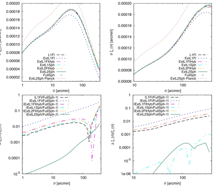
Figure 2. The difference of the two-point shear correlation functionsξ+(left) andξ−(right) of the ExtL2Sph projection relative to the full spherical case (FullSph). Two cases of the shear correlation function transformation for ExtL2Spha are shown, the full spherical case (equation 48, green solid lines), and the flat-sky Hankel transform (equation 47, red dashed curves).
The flat-sky shear power spectrumPγ can be related to the underlying matter power spectrum through equation (43) when adopting a first-order extended Limber approximation, or equation (44) when adopting a second-order extended Limber approximation.
On a sphere, correlation functions formally cannot be related to the power spectrum by the Hankel transform in equation (47), and should be replaced by the spherical transform (Ng & Liu1999; Chon et al.2004)
ξ+(θ)= 1
4π
∞
=2
(2+1)Cγ()d2 2 (θ); ξ−(θ)= 1 4π
∞
=2
(2+1)Cγ()d2−2(θ), (48)
where dm nare the reduced Wigner D-matrices (see Appendix C for details on their numerical calculation).
The spherical power spectrum is formally not defined for non-integer(see Castro et al.2005, for alternative spherical-sky formulae for the two-point correlation function), as functions defined on the sphere are necessarily periodic. As we have shown in Section 4.1, however, the spherical second-order extended Limber approximation provides a percent-level precision representation of the full spherical projection for >3. The spherical pre-factorł(, 2) (equation 18) can be generalized to non-integer arguments and is positive for≥2. We can thus use the spherical power spectrum with the Hankel transformation in equation (47) to compute the two-point correlation functions. This has the advantage being able to employ fast FFT numerical implementations of the Hankel tranforms (Hamilton2000), when Monte Carlo sampling. We compare predictions for the two-point shear correlation function using the Hankel transformation and the full spherical transformation in Fig.2. We show the full projection and the best approximation, ExtL2Sph. Note that for the ‘FullSph’ case we replace the full projection with ExtL2Sph for >200 to reduce computation time. We find that the Hankel transform (equation 47) is accurate to better than 5 (0.2) percent forξ+(ξ−). The difference between the second-order Limber and full projection solution using the spherical transform (equation 48) is well below one (0.03) percent on scales ofϑ <300 arcmin forξ+(ξ−). The red lines in Fig.2present the limit of precision that we can achieve with the current fast Hankel transform implementation for the correlation function. The green lines show the limit of the second-order Limber approximation on the correlation function.
Fig.3shows the two-point correlation functionsξ+(left) andξ−(right) using the different cases for the shear power spectrum listed in Table 1. The componentξ+ is calculated with the appropriate transformation, i.e. Hankel for the flat cases, and spherical involving Legendre polynomials for the spherical cases. Forξ−, which is less dominated by large scales and thus Limber and flat-sky approximations, in comparison toξ+, we use the Hankel transform in all cases. In addition, forξ−, the approximation ‘ExtL2Sph’ is our reference case. The adopted CFHTLenS redshift distribution and fiducial cosmological model are the same as in Fig.1. As is clear by the red dotted curve, using thePlanckcosmology (Planck Collaboration XIII2016) induces a significant change in the amplitude of the shear correlation function in comparison to the different projection methods.
4.3 Application to CFHTLenS data
Figure 3. The two-point shear correlation functionsξ+(left) andξ−(right). In the spherical cases (ExtL1Sph, ExtL2Sph, FullSph),ξ+andξ−have been computed using the spherical transform (equation 48). For the flat cases, the Hankel transform in equation (47) was used. The upper panels show the total shear correlation functions for the range of cases listed in Table1. The lower panels show the relative differences to the spherical sky second-order extended Limber approximation, ExtL2Sph. The theoretical models correspond to the CFHTLenS best-fitting cosmological parameters withm=0.279,h=0.701 and σ8=0.79 (Kilbinger et al.2013). For comparison, we also show, in the upper panels, the spherical sky second-order extended Limber approximation model for thePlanck-best fitting cosmology withm=0.3,h=0.67 andσ8=0.83 (Planck Collaboration XIII2016).
shape measurements (Miller et al.2013) and a full suite of informative systematic tests to select a clean data set (Heymans et al.2012). Since the public release of this survey in 2013, the community has continued to scrutinize and advance our understanding of CFHTLenS by identifying a number of areas where analyses could improve:
(i) Choi et al. (2016) identified significant biases in the tomographic photometric redshift distributions using a more effective clustering analysis, in comparison to Benjamin et al. (2013), by incorporating newly overlapping spectroscopic data from the Sloan Digital Sky Survey. The conclusion of this work was that any re-analysis of CFHTLenS should include systematic error terms to account for bias and scatter, with a prediction that accounting for these biases wouldreducethe recovered amplitude ofσ8by∼4 per cent. Additional new techniques to calibrate the redshift distribution of tomographic bins were introduced recently in Hildebrandt et al. (2017).
(ii) The CFHTLenS tomographic cosmological analysis was then revisited by Joudaki et al. (2017) in order to include a full redshift error analysis based on the results from Choi et al. (2016). The impact of correcting for these biases, including their associated errors, served to reduce the overall constraining power of the survey and hence also the tension between CFHTLenS and CMB constraints.
Table 2. Mean and 68 per cent credible interval forσ8(m/0.27)0.6and σ8(m/0.3)0.6for various approximations to the lensing power spectrum projections listed in Table1.
ID σ8(m/0.27)0.6 σ8(m/0.3)0.6
L1Fl 0.787+−00..033031 0.739+−00..029031
ExtL1Fl 0.792±0.032 0.744±0.030
ExtL1FlHyb 0.788−+00..031033 0.740+0
.029
−0.031 ExtL2FlHyb 0.788+−00..033031 0.740+−00..029031 ExtL2Sph(Hankel) 0.789+−00..032031 0.740+−00..029030
(iv) Kuijken et al. (2015) showed that the CFHTLenS shear calibration corrections derived in Miller et al. (2013) were underestimated as a result of an imperfect match between the galaxy populations in the data and image simulations.
(v) Fenech Conti et al. (2017) demonstrated that the CFHTLenS data would have been subject to a weight bias that favours galaxies that are more intrinsically oriented with the point-spread function. They also showed that the impact of calibration selection biases, which were not considered in Miller et al. (2013), would have lead to the overcorrection of multiplicative shear bias in the CFHTLenS analyses, by a few percent.
(vi) Joudaki et al. (2017) updated the CFHTLenS covariance matrices using larger box numerical simulations that were less subject to the lack of power on large scales. A complementary accurate estimate of the covariance matrix using analytical methods will be published soon (Joachimi et al., in preparation)
(vii) Takahashi et al. (2012) provided a more accurate non-linear power spectrum correction than that used in the original CFHTLenS analyses, and the halo model from Mead et al. (2015) allowed for simultaneous modelling of baryonic modifications to the non-linear power spectrum.
All these advances in our understanding were incorporated and accounted for in the recent KiDS cosmic shear analysis (Hildebrandt et al.2017), which reports a 2.3σ tension withPlanck. Efforts are now underway to fully re-analyse CFHTLenS using the advanced KiDS analysis pipeline with revised shape measurements and calibrations for the shear and photometric redshifts. Until this analysis is complete, we note that these known shortcomings with the original CFHTLenS results impact in different ways the cosmological conclusions that one can draw. As CFHTLenS has similar statistical power to current weak-lensing surveys, however, it nevertheless provides a very useful testbed with which to demonstrate the impact of adopting different approximations when constraining cosmological parameters.
In this work, we focus on the weak-lensing power spectrum projection, and assess the impact of various approximations on cosmological constraints from CFHTLenS. For consistency with the original analysis (Kilbinger et al.2013), we adopt the same priors and non-linear power spectrum corrections from Smith et al. (2003).
We re-analyse the 2D CFHTLenS measurement of the two-point shear correlation functionξ±(θ) from Kilbinger et al. (2013), defined in equation (47). As in Kilbinger et al. (2013), we fit both componentsξ+andξ−between angular scalesθ=0.8 and 350 arc min, and use a N-body simulation estimate of the non-Gaussian covariance including the cross-covariance between both components. Bayesian Population Monte Carlo parameter sampling is performed using the publicly available software COSMOPMC5(Wraith et al.2009; Kilbinger et al.2010). The cosmological modelling part includes the various lensing projections, calculated using the software libraryNICAEA.6
For a first-order standard Limber flat-sky approximation (L1Fl), we find σ8(m/0.27)0.6=0.787+−00..031033, the same result that was published in Kilbinger et al. (2013). Using the second-order extended Limber flat-sky hybrid approximation (ExtL2FlHyb) results in σ8(m/0.27)0.6 =0.788±0.032, a negligible change of the amplitude that is well within the Monte Carlo sampling noise. The largest difference is measured with the deprecated case ExtL1Fl, for which the recovered amplitude is larger by 16 per cent of the statistical error. These negligible changes to the error bars were to be expected owing to the high level of statistical noise and cosmic variance in comparison to the low-level impact of the various approximations shown in Fig.1.
Table2lists the mean and 68 per cent credible interval forσ80m.6for the various approximations to the lensing power spectrum projections listed in Table1. Note again that these values do not represent the state-of-the-art cosmological results, since many of the above listed analysis advancements made since 2013 have not been taken into account. As an example of a significant effect, when using the revised non-linear power spectrum of Takahashi et al. (2012) in place of Smith et al. (2003), there is a decrease of 0.6σ withσ8(m/0.27)0.6=0.768+−00..029031, using L1Fl.
Considering the cosmological constraints from tomographic Kilo-Degree Survey (KiDS), we conclude that these are robust to flat-sky and Limber approximations. The case ExtL1FlHyb that was used for the analysis of KiDS data in Hildebrandt et al. (2017) and Joudaki et al. (2016) introduces errors that are more than an order of magnitude lower than the cosmic variance for that survey, and thus this approximation has a negligible impact on the cosmological parameters.
Figure 4. Integrand ofξ+(upper),ξ−(upper middle),E1(lower middle, E-COSEBIs) andMap2(lower panel). All integrands are of the formF()P(), whereF() is the corresponding weight-function for each statistic andP() is the E-mode convergence power spectrum, with the exception ofξ±, for which
P() is equal to the sum of the E and B-mode power spectra. Two cases are shown for each statistic as listed in each caption. For the aperture mass statistic, θmax=2θis shown. Note that higher order COSEBIs modes generally probe larger-modes, hence here we show only the lowest modeE1. All values are normalized with respect to their maximum value. This figure illustrates how different two-point cosmic shear statistics have different dependences between the angular scales sampled and the-range probed.
4.4 Alternative two-point shear statistics; the mass aperture statistic and COSEBIs
The two-point shear correlation functionξ±represents the current baseline observable for cosmic shear measurements. As shown in Fig.3, however, using the standard first-order extended Limber flat-sky approximation (ExtL1FlHyb) can result in errors exceeding 10 per cent, on angular scalesθ >300 arcmin. This is a result of the weight given to lowmodes in theξ+statistic, as illustrated in Fig.4, which shows the integrand ofξ+andξ−(upper two panels) for two cases(θ=100 and 350 arcmin), normalized to their maximum value. This error does not impact CFHTLenS analyses, given the low signal to noise of the measurements on these scales. It will however become increasingly important for upcoming wider field surveys that will accurately probe these scales.
In this paper, we provide a solution in the form of the second-order extended Limber approximation, but another option to consider is the use of alternative two-point shear statistics that are less sensitive to accuracy in shear power spectrum measurement at low. Both the aperture-mass dispersion,Map2 (Schneider et al.1998), and the Complete Orthogonal Sets of E/B-mode Integrals (COSEBIs),E
n(Schneider et al.2010) statistics satisfy this requirement and are linearly related to the shear power spectrum in the flat-sky approximation via integrals of the form
Map2 (θ)= 1
2π
∞
0
d Uˆ2(θ)Pγ(), (49)
En= 1
2π
∞
0
d Wn()Pγ(), (50)
for the lowest COSEBIs mode,E1, as the higher modes generally probe larger-modes. The lowest panel shows the integrands of aperture mass dispersion statistics, for the same two maximum angular ranges.
Note that the development of the aperture-mass dispersion statistic,Map2 , was initially motivated to enable the separation of the measured signal into an E-mode (cosmological signal) and B-mode (systematics). This statistic is, however, a lossy conversion and is biased by small angular separations, where blending of galaxies makes shear measurement challenging (Kilbinger, Schneider & Eifler2006). The COSEBIs statistic tackles both these shortcomings. Kilbinger et al. (2013) present a detailed comparison of cosmological constraints obtained from this range of different two-point shear statistics finding consistent results.
5 C O N C L U S I O N S
In this paper, we evaluate precision theoretical calculations for cosmic shear observables, bringing together different sources from the literature to provide a pedagogical review of the impact of adopting flat-sky and Limber approximations. We demonstrate that for current surveys, such as CFHTLenS and KiDS, these approximations have a negligible impact on cosmological parameter constraints.
For future surveys, the decrease in statistical errors places higher requirements on the accuracy of the theoretical modelling. There is also, however, the need to be able to rapidly sample the multidimensional cosmological parameter likelihoods. This requirement for computational speed is incompatible with a theoretical analysis that calculates a full spherical solution for the shear power spectrum, without adopting any approximation. We therefore present alternative solutions, revisiting the work of Bernardeau et al. (2012), who showed that adopting the second-order extended Limber approximation of Loverde & Afshordi (2008) provides a representation of the full spherical solution for the shear power spectrum that is accurate at the sub-percent level for >3. We have verified this result and provide to the community our fast numerical implementation of all the approximations studied in this analysis, and the slow calculation of the full projection within the publicly available packageNICAEAathttp://www.cosmostat.org/software/nicaea.
Finally, we propose that future surveys seek to optimize the statistical analyses of their cosmic shear data. For example, moving from the standard two-point shear correlation function statistic to the more stringent ‘COSEBI’ statistic (Schneider et al.2010) renders the cosmic shear measurement insensitive to the low-scales where the Limber and flat-sky approximations have an impact on the precision of the theoretical modelling.
We have considered a flat universe throughout this paper. To generalize the calculations to non-flat models, one needs to modify the comoving angular diameter distance to account for the spatial curvatureK=0. In addition, the spherical Bessel functions are replaced with hyperspherical Bessel functions (Abbott & Schaefer1986). In a universe with positive curvatureK>0, the 3D wave modes become discrete integer variables. For non-flat models, we do however not expect qualitative differences from our results.
AC K N OW L E D G E M E N T S
The authors thank Tommaso Giannantonio, Sarah Bridle, Ami Choi, Donnacha Kirk, Lance Miller, Benjamin Joachimi, Chris Blake, Joe Zuntz, Joanne Cohn, Alex Hall and Adam Amara for very helpful discussions. This work was financially supported by the Deutsche Forschungsgemeinschaft (DFG) (Emmy Noether grant Hi 1495/2-1; SI 1769/1-1; TR33 ‘The Dark Universe’), the Alexander von Humboldt Foundation, the European Research Council (ERC) (grants 279396, 647112), the Seventh Framework Programme of the European Commission (Marie Sklodwoska Curie Fellowship grant 656869), the Netherlands Organization for Scientific Research (NWO) (grants 614.001.103), Natural Sciences and Engineering Research Council of Canada (NSERC), Canadian Institute for Advanced Research (CIfAR) and the World Premier International Research Center Initiative (WPI), Ministry of Education, Culture, Sports, Science and Technology (MEXT), Japan. Parts of this research were conducted by the Australian Research Council Centre of Excellence for All-sky Astrophysics (CAASTRO), through project number CE110001020i, and by the German Federal Ministry for Economic Affairs and Energy (BMWi) under project no. 50QE1103.
R E F E R E N C E S
Abbott L. F., Schaefer R. K., 1986, ApJ, 308, 546 Abbott T. et al., 2016, Phys. Rev. D, 94, 022001
Asgari M., Heymans C., Blake C., Harnois-Deraps J., Schneider P., Van Waerbeke L., 2017, MNRAS, 464, 1676 Bartelmann M., Schneider P., 2001, Phys. Rep., 340, 291
Benjamin J. et al., 2013, MNRAS, 431, 1547 Bernardeau F., 1998, A&A, 338, 375
Bernardeau F., Bonvin C., Van de Rijt N., Vernizzi F., 2012, Phys. Rev. D, 86, 023001 Blanco M. A., Fl´orez M., Bermejo M., 1997, J. Mol. Struct., 419, 19
Castro P. G., Heavens A. F., Kitching T. D., 2005, Phys. Rev. D, 72, 023516 Choi A. et al., 2016, MNRAS, 463, 3737
Chon G., Challinor A., Prunet S., Hivon E., Szapudi I., 2004, MNRAS, 350, 914 Erben T. et al., 2013, MNRAS, 433, 2545
Fenech Conti I., Herbonnet R., Hoekstra H., Merten J., Miller L., Viola M., 2017, MNRAS, 467, 1627 Fu L. et al., 2008, A&A, 479, 9
Hamana T., Colombi S. T., Thion A., Devriendt J. E. G. T., Mellier Y., Bernardeau F., 2002, MNRAS, 330, 365 Hamilton A. J. S., 2000, MNRAS, 312, 257
Heymans C. et al., 2012, MNRAS, 427, 146 Hildebrandt H. et al., 2012, MNRAS, 421, 2355 Hildebrandt H. et al., 2017, MNRAS, 465, 1454 Hu W., 2000, Phys. Rev. D, 62, 043007
Jee M. J., Tyson J. A., Schneider M. D., Wittman D., Schmidt S., Hilbert S., 2013, ApJ, 765, 74 Joudaki S., Kaplinghat M., 2012, Phys. Rev. D, 86, 023526
Joudaki S. et al., 2016, MNRAS, 471, 1259 Joudaki S. et al., 2017, MNRAS, 465, 2033 Kaiser N., 1992, ApJ, 388, 272
Kaiser N., 1998, ApJ, 498, 26
Kilbinger M., Schneider P., Eifler T., 2006, A&A, 457, 15 Kilbinger M. et al., 2010, MNRAS, 405, 2381
Kilbinger M. et al., 2013, MNRAS, 430, 2200
Kitching T. D., Heavens A. F., 2016, Phys. Rev., 95, 063522
Kitching T. D., Alsing J., Heavens A. F., Jimenez R., McEwen J. D., Verde L., 2016, MNRAS, 469, 2737 Kuijken K. et al., 2015, MNRAS, 454, 3500
Lemos P., Challinor A., Efstathiou G., 2017, J. Cosmol. Astropart. Phys., 5, 014 Limber D. N., 1953, ApJ, 117, 134
Loverde M., Afshordi N., 2008, Phys. Rev. D, 78, 123506
Mead A. J., Peacock J. A., Heymans C., Joudaki S., Heavens A. F., 2015, MNRAS, 454, 1958 Miller L. et al., 2013, MNRAS, 429, 2858
Miralda-Escude J., 1991, ApJ, 370, 1
Ng K.-W., Liu G.-C., 1999, Int. J. Mod. Phys. D, 8, 61
Peebles P. J. E., 1980, The Large-Scale Structure of the Universe. Princeton Univ. Press Planck Collaboration XIII, 2016, A&A, 594, A13
Schmidt F., 2008, Phys. Rev. D, 78, 043002
Schneider P., Van Waerbeke L., Jain B., Kruse G., 1998, MNRAS, 296, 873 Schneider P., Van Waerbeke L., Mellier Y., 2002, A&A, 389, 729 Schneider P., Eifler T., Krause E., 2010, A&A, 520, A116 Smith R. E. et al., 2003, MNRAS, 341, 1311
Takahashi R., Sato M., Nishimichi T., Taruya A., Oguri M., 2012, ApJ, 761, 152 Taylor A. N., 2001, Phys. Rev. Lett, submitted in press
Van De Rijt N., 2012, PhD thesis, ´Ecole Polytechnique
Wraith D., Kilbinger M., Benabed K., Capp´e O., Cardoso J.-F., Fort G., Prunet S., Robert C. P., 2009, Phys. Rev. D, 80, 023507
A P P E N D I X A : D E R I VAT I O N O F T H E W E A K - L E N S I N G P OW E R S P E C T R A
The following derivations are detailed in Hu (2000) and Castro et al. (2005), and are provided here for completeness.
A1 Spherical case
A1.1 Lensing potential power spectrum
To obtain the power spectrum of the lensing potential, we insert the lensing projection (equation 1) into the inverse harmonics expansion (equation 7) and write the 3D potential as its Fourier transform (equation 5) to get
ψm= c22
dY∗m(θ, ϕ)
∞
0 dχ
χ q(χ)
d3k
(2π)3ˆ(k;χ)e
−ik·r.
(A1)
The 3D position vectorris a 3D position vector with polar coordinater=χand polar angles (θ,ϕ). Similarly, we denote withθk,ϕkthe polar angles of the 3D Fourier vectork. We insert the expansion of a plane wave into spherical harmonics,
eik·r=4π
∞
=0
m=−
ij(kχ)Ym(θ, ϕ)Ym(θk, ϕk). (A2)
Making use of the orthogonality of the spherical harmonics
dYm(θ, ϕ)Y∗m(θ, ϕ)=δδmm, (A3)
the expression forψmsimplifies to
ψm= i
c2π2
∞
0 dχ
χ q(χ)
d3kˆ(k;χ)j(kχ)Ym(θk, ϕk). (A4)
coordinates, d3k=dkk2d
kand use once again the orthogonality of the spherical harmonics to resolve the spherical integral. This leads to the potential power spectrum in equation (9).
A P P E N D I X B : D I S C U S S I O N A N D C O M PA R I S O N T O P R E V I O U S LY P U B L I S H E D W O R K
In this section, we briefly discuss previously published work on the full projection and second-order Limber equation of the lensing power spectrum, cross-checking and comparing their results with our independent findings.
B1 Kitching et al.2016(version 1)
Kitching et al. (2016) compute the full projection of the weak-lensing power spectrum, which they present as spherical-radial representation of the 3D shear field. Our results in equation (21) correspond to their equations (7) and (8) assuming a flat universe and the case of perfect photometric redshifts, withp(z|zp)=δD(z−zp), and for a bin function that selects the redshift bin ofz,WSR(z,zp) is unity ifzpis in the redshift bin denoted byz, and zero otherwise. We find that equation (7) in Kitching et al. (2016) is missing a factor 2/π.
Kitching et al. (2016) derive the spherical and extended Limber approximation starting from the full spherical projection in their Appendix A. We find that the filter functionqdefined in their equation (31) has an additional factor of comoving distancer, and an additional factor ofπ/2.
As shown in this paper, we are unable to reproduce the differences that Kitching et al. (2016) report, between the full spherical solution and the different approximations, neither for the power spectrum nor for the shear correlation function.
B2 Bernardeau, Bonvin, Van de Rijt, Vernizzi (2012); Van de Rijt (2012)
Bernardeau et al. (2012) present the non-tomographic full projectionC() in the approximation of the 3D potential power spectrumP
separating intok- andχ-dependent functions in their equation (44). Their expression holds for a single source redshift.
The PhD thesis of Van De Rijt (2012) presents an explicit calculation of the second-order Limber approximation. They carry out the derivatives of the kernelsfunder the assumption of a constant growth-suppression factorD+(a)/a. Then, for a constant source comoving distanceχS, the lensing efficiency in equation (2) isq(χ)=(χS−χ)χS−1, and the derivative of the separated kernel function in equation (41) can be calculated analytically,
f
s(χ)+
χ 3f
s (χ)= − 1 8χ
−5/2
5 χ +
1 χS
D+(χ)
a(χ) . (B1)
This result confirms the power-law behaviour forχχSof the filter function, which we exploited earlier to fit this function.
Inserting equation (B1) into the second-order Limber power spectrum in equation (42) and using the inverse Poisson equation to replace the matter with the potential power spectrum, we obtain the same expression as Van De Rijt (2012) (their equation 7.19).
In Fig.B1, we reproduce fig. 7.3 from Van De Rijt (2012) using a similar set up, a flatUniverse withm=0.3,h=0.65,b=0.0461,
σ8=0.8,ns=0.96. All source galaxies are at redshiftzS=1. The non-linear 3D matter power spectrum from Takahashi et al. (2012) is used. The ratio of the first-and second-order Limber approximated power spectra to the full projection shows excellent agreement at the sub-percent level.
B3 LoVerde & Afshordi (2009)
This paper introduces the extended Limber approximation to second order that we apply in this work. Although they present the specific case of 2D galaxy clustering, their calculations are general enough to apply to a weak-lensing context. Their equation (5) is a spherical cross-power spectrum of two scalar fieldsAandB, projected from 3D to 2D via projection kernelsFAandFBdefined in their equation (4). Comparing their expressions with the weak-lensing potential (1), we setFA(χ)=FB(χ)=2c−2D+(χ)q(χ)χ−1. With that, their equation (5) is identical to equation (9).
The second-order Limber approximation in Loverde & Afshordi (2008) is presented in equation (12). This is consistent with our first-order (equation 38) and second-order (equation 39) Limber approximation terms, when accounting for the difference between lensing potential and shear 2D power spectrum, and 3D potential and matter power spectrum.
B4 Schmidt (2009)
Schmidt (2008) derive the lensing power spectrum in the flat-sky limit (see their equation 9). Inserting the Poisson equation and the growth function, and writing the redshift filter functionWκ(eq. 10) in terms of the lensing efficiency and comoving distances,Wκ[z(χ)]=H(z)−1χq(χ),
their expression, using our notations, reads
Pijγ()=
2
π A2 ∞
0
dχχ qi(χ) a(χ)
∞
0
dχχqj(χ
) a(χ)
∞
0
dk k2P